8.2.Contingency Analyses

2x2 chi-2, Fisher| Acknowledgments to Y. Brandvain for code used in some slides

Bárbara D. Bitarello

2025-11-26

Outline

• Quantifying associations between two categorical variables

• Relative risk

• Odds-ratio

• OR vs RR

• Testing associations between categorical variables

• \(\chi^2\) contingency test

• Fisher’s test

Recap

Contingency analysis estimates and tests for an association between two or more categorical variables.

• At the heart of these approaches we are really investigating the independence of variables

RR vs OR

• Both \(RR\) and \(OR\) measure the association between two categorical variables when both have only 2 categories.

• RR is the probability of an undesired outcome in the treatment group divided by the probability of the same outcome in a control group. Especially appropriate when comparing the probability (risk) of a focal outcome in a response variable between two treatments or groups of subjects

• The OR is the odds of “success” (focal outcome) in one group divided by the odds of success in a second group. The explanatory variable defines the groups being compared.

• E.g. death in the titanic for women x men. Focal outcome is death. “Treatment” group for RR is women

When to Calculate OR (1/2)?

We often cannot obtain an unbiased estimate of \(p_1\) or \(p_2\).

Odds ratios risk can be calculated even when we don’t have a random sample and we can’t obtain unbiased probabilities!

Thus it is extremely useful for “case-control” studies, as they have a large sample of individuals with rare conditions.

\[\widehat{OR} = \frac{\widehat{O_1}}{\widehat{O_2}} = \frac{a/c}{b/d} = \frac{ad}{bc}\]

	Treatment	Control
Success (focal outcome)	a	b
Failure (alternative outcome)	c	d

Case control studies: an observational study in which a sample of individuals with a focal condition (cases) is compared to a sample of subjects lacking the condition (controls).

Odds Ratio: Toxoplasma & Car Wrecks

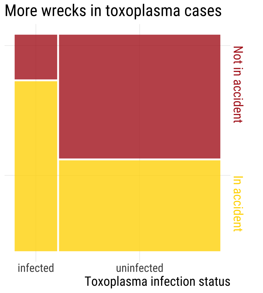
Toxoplasma tricks mice into taking risks so it can find it’s way into cats. Could Toxoplasma be associated with risk taking in humans? Yereli et al. asked this by comparing Toxoplasma prevalence in people who caused car crashes to those who hadn’t.

\(\widehat{OR}\): Toxoplasma & Car Wrecks. Try!

	Treatment	Control
Success (focal outcome)	a	b
Failure (alternative outcome)	c	d

\[\widehat{OR} = \frac{\widehat{O_\text{infected}}}{\widehat{O_\text{uninfected}}} = \frac{a/c}{b/d} = \frac{ad}{bc} = ??? \]

	infected	uninfected
In accident	61	124
Not in accident	16	169

\(\widehat{OR}\): Toxoplasma & Car Wrecks

	Treatment	Control
Success (focal outcome)	a	b
Failure (alternative outcome)	c	d

\[\widehat{OR} = \frac{\widehat{O_\text{infected}}}{\widehat{O_\text{uninfected}}} = \frac{a/c}{b/d} = \frac{ad}{bc} =\frac{61 \times 169}{124 \times 16} = 5.2\]

	infected	uninfected
In accident	61	124
Not in accident	16	169

Toxoplasma & Car Wrecks. Summary

Without knowing the \(P(wreck \| toxoplasma)\) and \(P(wreck \| w/out toxoplasma)\) we can’t estimate RR

Still, we learned that the odds of being in a car wreck is five times higher if you have toxoplasma than if you do not!

Toxoplasma & Car Wrecks. Uncertainty

We estimate that the odds of being in a car wreck is 5.2 for those with, than those without Toxoplasma.

We know that estimates are associated with uncertainty.

We can quantify this!

Toxoplasma & Car Wrecks: OR 95% CI [1/2]

1st know that that standard error for the odds ratio cannot be directly computed, but the standard error of the log odds can!

\[SE[ln(\widehat{OR})] = \sqrt{\frac{1}{a} + \frac{1}{b} + \frac{1}{c} + \frac{1}{d}}\]

Then to find the 95% CI

1. Calculate \(SE[ln(\widehat{OR})]\)

2. Find the confidence limits of the log-odds as \(SE[ln(\widehat{OR})] \pm 2 \times SE[ln(\widehat{OR})]\)

3. Exponentiate this result to get back to linear scale

Toxoplasma & Car Wrecks: OR 95% CI [2/2]

1. \(SE[ln(\widehat{OR})] = \sqrt{\frac{1}{61} + \frac{1}{124} + \frac{1}{16} + \frac{1}{169}} = 0.305\)

2. Find the 95% CI as \(ln(\widehat{OR}) \pm 2 \times SE[ln(\widehat{OR})]\)
   \(= ln(5.2) \pm 2 \times 0.305\)
   \(= 1.65 \pm 0.61\)
   95% CI of \(ln(\widehat{OR})\) is between 1.04 and 2.26

3. 95% CI of \(\widehat{OR}\) = exp(c(1.04, 2.26)) = 2.8, 9.6

CONCLUSION: \(2.8 < OR < 9.6\)
The odds of getting in an accident are plausibly between 2.8 and 9.6 times higher for people with than without Toxoplasma.
- Because the 95% CI does not contain 1, we reject the null hypothesis and conclude that there is an association between Toxoplasma infection and car accidents.

In R

The easiest way to calculate OR and CIs in R:

toxoplasma <- matrix(c(61, 16, 124, 169), nrow = 2)
colnames(toxoplasma) <- c("inf", "not-inf")
rownames(toxoplasma) <- c("crash", "no_crash")
toxoplasma
##          inf not-inf
## crash     61     124
## no_crash  16     169
fisher.test(toxoplasma, conf.int = T)
## 
##  Fisher's Exact Test for Count Data
## 
## data:  toxoplasma
## p-value = 8e-09
## alternative hypothesis: true odds ratio is not equal to 1
## 95 percent confidence interval:
##   2.79 10.09
## sample estimates:
## odds ratio 
##       5.17

The CI above is a little different from the one before (Wald method) because this function uses a different method. You can find out more in the help(fisher.test) function. Lab10 also goes over this.

RR 95% CI

The 95% CI for the RR is also not pretty. Based on the same assumptions as the one we showed for \(OR\) (i.e., random samples):

\[SE[ln(\widehat{RR})] = \sqrt{\frac{1}{a} + \frac{1}{b} - \frac{1}{a+c} - \frac{1}{b+d}}\]

\[ln(\widehat{RR})-2\times SE[ln(\widehat{RR})]<ln(RR) < ln(RR)+2\times SE[ln(\widehat{RR})]\]

Note that for \(RR\) and \(OR\) there are several available methods and no consensus over which one is best.

The two we showed here use a type of rule of thumb based on the normal distribution. I.e., these are approximations based on the Z distribution.

95% CI in R with resampling (instead of this dreadful equation)

• There is another way: we can bootstrap!

• By bootstrapping, we approximate the sampling distribution by resampling outcomes with replacement and summarizing variability in this resampling to describe uncertainty.

Testing Associations Between Categorical Variables

\(\chi^2\) Contingency Tests and Fisher’s Exact Test

\(\chi^2\) Contingency Test of Independence

Remember: The multiplication rule states that if two outcomes, A & B are independent, \[P[A \& B] = P[A] \times P[B]\]

• So, we have our expectation under the null hypothesis that A & B are independent.

• We can test if our deviation from this expectation is unexpected under the null from the \(\chi^2\) test!

• This is imply a special case of the \(\chi^2\) goodness of fit where the model described the independence between two (or more) categorical variables

Calculating \(\chi^2\) & Degrees of Freedom

Remember: \(\chi^2\) is the sum of deviations between expectations and observations,\(i\) and \(j\) are rows and columns, respectively.

\[\sum_i \sum_k{\frac{{(\text{Observed}_{i,j}-\text{Expected}_{i,j})^2}}{\text{Expected}_{i,j}}}\]

• The degrees of freedom specify the additional number of values we need to know all the outcomes in our study.

• \(\text{Degrees of freedom for } \chi^2 \text{ contingency test} = (n_\text{rows} - 1) \times (n_\text{columns} - 1)\)

Bird Abandonment Issues [1/]

What’s a bird to do when the rent is do and they can’t feed their chicks?

Kloskowski tested the idea that birds in poor habitats abandon their final egg.

Data for this example: Data for this example: https://doi.org/10.5061/dryad.6k417tm

Bird Abandonment Issues [2/]

Bird Abandonment Issues [3/]

Hypotheses:

\(H_0\): There is NO association between habitat quality & the chance of abandoning the last egg

\(H_A\): There is AN association between habitat quality & the chance of abandoning the last egg

Bird Abandonment Issues [4/]

Observations (contingency table)

table(birds$`Last egg`, birds$`Habitat quality`) |>
    kable()

	High	Low
Abandoned	1	19
Hatched	53	21

Bird Abandonment Issues [5/]

Observations (contingency table)

	High	Low	Total
Abandoned	1	19	20
Hatched	53	21	74
Total	54	40	94

Find null expectations!!!!!!

\(n_{abandoned}=(1+19)=20\)

\(n_{\text{hatched}}=74\)

Bird Abandonment Issues [6/]

Multiply proportions by each other and sample size to find null expectations. \[E[n(A,B) | n] = n \times P[A] \times P[B]\]

Habitat quality	Last egg	observed	n.habitat	n.egg
High	Abandoned	1	54	20
High	Hatched	53	54	74
Low	Abandoned	19	40	20
Low	Hatched	21	40	74

\(P_{habitat}=n_{habitat}/n_{total}\)

\(P_{egg}=n_{egg}/n_{total}\)

E.g. Expected \(P(\text{high & abandoned})=0.574\times 0.213\times 94\)

Bird Abandonment Issues [7/]

Null expectations:

Multiply proportions by each other and sample size to find null expectations. \[E[n(A,B) | n] = n \times P[A] \times P[B]\]

Abandonment: \(\chi^2\) Assumptions?

Remember assumptions

• No more than 20% of categories have Expected \(< 5\)

• No category with Expected \(\leq 1\)

Habitat quality	Last egg	observed	p.habitat	p.egg	expected
High	Abandoned	1	0.574	0.213	11.49
High	Hatched	53	0.574	0.787	42.51
Low	Abandoned	19	0.426	0.213	8.51
Low	Hatched	21	0.426	0.787	31.49

We meet the assumptions

Abandonment: \(\chi^2\)

Remember: \(\chi^2\) is the sum of the squared deviations from expected counts divided by expected counts.

\[\sum \frac{(\text{Observed}-\text{Expected})^2}{\text{Expected}}\]

\[\frac{( 1-11.5)^2}{11.5} + \frac{( 53-42.5)^2}{42.5} + \frac{( 19-8.5)^2}{8.5} + \frac{( 21-31.5)^2}{31.5}\]

So \(\chi^2 = 28.59\)(without rounding anywhere)

\[df = (n_\text{columns} - 1) \times (n_\text{rows} - 1)\]

\[df = (2 - 1) \times (2 - 1) = 1\]

Abandonment: Critical & P-values

Critical value at for df in rows and alpha level in columns

	0.1	0.01	0.001	1e-04	1e-05	1e-06	1e-07	1e-08
df = 1	2.7	6.6	10.8	15.1	19.5	23.9	28.4	32.8
df = 2	4.6	9.2	13.8	18.4	23.0	27.6	32.2	36.8

We’re significant at the \(1e-7\) level

We reject the \(H_0\) and conclude that bird abandon eggs in bad environemnts.

In R: pchisq(q = birds.chi, df = 1, lower.tail = FALSE)
= 8.96e-08

One tailed test?

Note that we only looked at one tail of the \(\chi^2\) distribution.

This does not mean that we only notice an association in one direction.

Both ways to be exceptional (an association between abandonment and poor environments OR an association between abandonment and good environments) yield a strong discrepancy between observations and expectations, and can generate a significant association.

Always quantify effect size, direction, and uncertainty

Bird abandonment with OR and CI

	High	Low
Abandoned	1	19
Hatched	53	21

\(OR=(1*21)/(53*19)=0.0209\)

# OR in this function is calculated a bit differently, hence the difference.
fisher.test(tab2)
## 
##  Fisher's Exact Test for Count Data
## 
## data:  tab2
## p-value = 5e-08
## alternative hypothesis: true odds ratio is not equal to 1
## 95 percent confidence interval:
##  0.000499 0.153059
## sample estimates:
## odds ratio 
##     0.0217

OR 95% CI: \(0.0005 <OR < 0.153\), reject the null.

What if we don’t meet \(\chi^2\) requirements?

Example: Nuptial Gifts

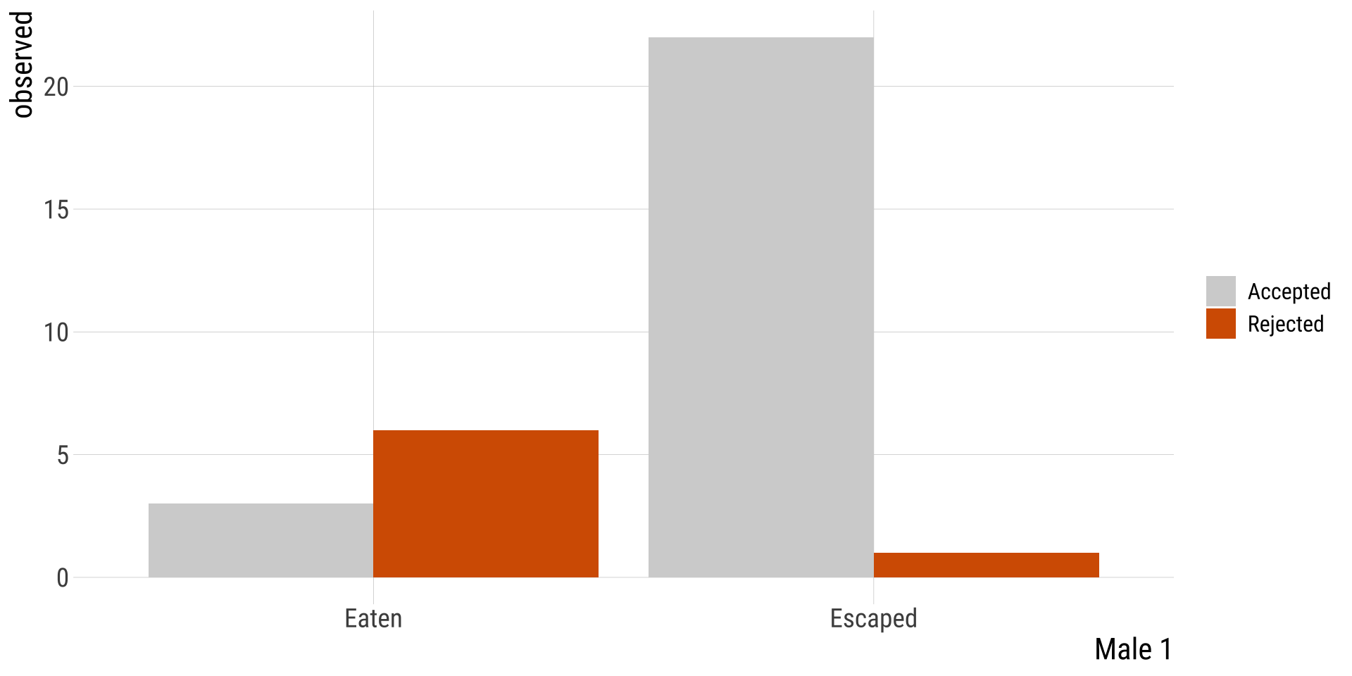
Sometimes, females of the Australian redback spider Latrodectus hasselti eat there mates. Is there anything in it for the males?

Maydianne Andrade tested the idea that eating a male might distract a female & prevent her for remating with a \(2^\text{nd}\) male.

Example from: Andrade, M. (1996). Science 271: 70-72 link

Nuptial Gift: Observed & Expected

Male_2	Male_1	observed
Accepted	Eaten	3
Rejected	Eaten	6
Accepted	Escaped	22
Rejected	Escaped	1

Nuptial Gift: \(\chi^2\) Assumptions?

• No more than 20% of categories have Expected \(< 5\)

• No category with Expected \(\leq 1\)

We do not meet assumptions

Male_2	Male_1	observed	p.Male1	p.Male2	expected
Accepted	Eaten	3	0.28	0.78	7.03
Rejected	Eaten	6	0.28	0.22	1.97
Accepted	Escaped	22	0.72	0.78	17.97
Rejected	Escaped	1	0.72	0.22	5.03

Fisher’s Exact Test

• Generates all possible permutations of your data.

• Asks what proportion of configurations result in associations as or more extreme than observed.

\(p-value =\)(Sum of Probabilities of Tables at least as Extreme as Observed Table) / (Sum of Probabilities of All Possible Tables)

The test statistic is calculated based on the hypergeometric distribution (which we won’t go into), which gives the probability of observing the given contingency table under the assumption of independence.

Fisher’s test in R

fisher.test(spider.spread)
## 
##  Fisher's Exact Test for Count Data
## 
## data:  spider.spread
## p-value = 6e-04
## alternative hypothesis: true odds ratio is not equal to 1
## 95 percent confidence interval:
##  0.000482 0.329721
## sample estimates:
## odds ratio 
##     0.0279

	method	lower.95	upper.95	odds_ratio	p.value
odds ratio	Fisher's Exact Test for Count Data	5e-04	0.3297	0.0279	6e-04

We reject the null hypothesis.

Doing our own permutations

\(1^{st}\) tidy data by going from this on left, to this on right

Male_2	Male_1	observed
Accepted	Eaten	3
Rejected	Eaten	6
Accepted	Escaped	22
Rejected	Escaped	1

Male_2	Male_1
Accepted	Eaten
Accepted	Eaten
Accepted	Eaten
Rejected	Eaten
Rejected	Eaten
Rejected	Eaten
Rejected	Eaten
Rejected	Eaten
Rejected	Eaten
Accepted	Escaped
Accepted	Escaped
Accepted	Escaped
Accepted	Escaped
Accepted	Escaped
Accepted	Escaped
Accepted	Escaped
Accepted	Escaped
Accepted	Escaped
Accepted	Escaped
Accepted	Escaped
Accepted	Escaped
Accepted	Escaped
Accepted	Escaped
Accepted	Escaped
Accepted	Escaped
Accepted	Escaped
Accepted	Escaped
Accepted	Escaped
Accepted	Escaped
Accepted	Escaped
Accepted	Escaped
Rejected	Escaped

By doing this

disaggregated.spider <- spider %>%
    uncount(weights = observed)

Chi-squared vs Fisher’s exact test

• Both have the same null hypothesis: the outcome is independent from the groups.
• Chi-square is generally best for larger samples and Fisher’s is better for smaller samples.
• Both can be extended to cases beyond 2x2 with 2 categorical variables, such as 3x2, 2x5, etc
• When to use Fisher’s exact test:

1. 20% of categories with Expected values < 5

2. Any expected value <1
3. The column or row marginal values are extremely uneven.

• Note: Fisher’s ok for all sample sizes. But the # of possible tables grows at an exponential rate and soon becomes unwieldy. So mostly used for smaller sample sizes.