2.2.Displaying & Describing Data

Measures of central tendency and spread

Bárbara D. Bitarello

2025-09-17

Last time

• Mean
• Median

today: location and width; next class plots

Today

• Median example
• Mode
• Estimates of width
• Explanatory and exploratory figures
• Best practices in figure design
• How data types drive figure design
• How to make effective tables

Attention

Estimate = \(\bar{Y}, \bar{x}, \text{etc.}\) (sample mean)

• Variable

Parameter = \(\mu\) (population mean) - Constant

Practice: Median with even sample size

Calculate the median of the following 10 numbers: \(12, 2, 9, 18, 4, 1, 10, 19, 14, 17\)

Mean x Median

• The mean is more convinient mathematically.

• The mean is the center of gravity

• The median is a better descriptor for skewed population distributions.

• The median is the middle measurement.

Both can lead to values that don’t actually exist in the sample. E.g., the average number of eggs laid by chickens in a farm might be 5.5 and the median number of children millennials have might be 1.2

Case Study

2005 U.S. Census. The plot shows the income per household distribution for the bottom 98% of the population. Median = \(\sim46\)k; Mean: \(\sim63\)k.

From: https://www.visualizingeconomics.com/blog/2006/11/05/2005-us-income-distribution

For measures like income, medians are generally preferable to means. Why? Populations are right-skewed (there are few very rich people), and we care more about the average person than the average of people.

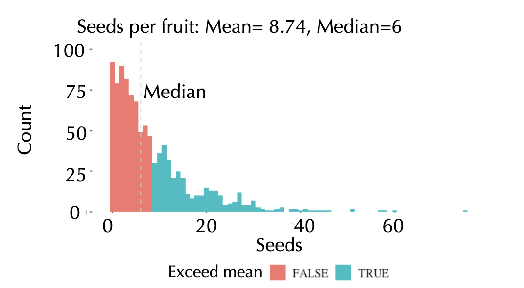
Mean or Median?

Number of seeds per fruit. Which one is better in this case?

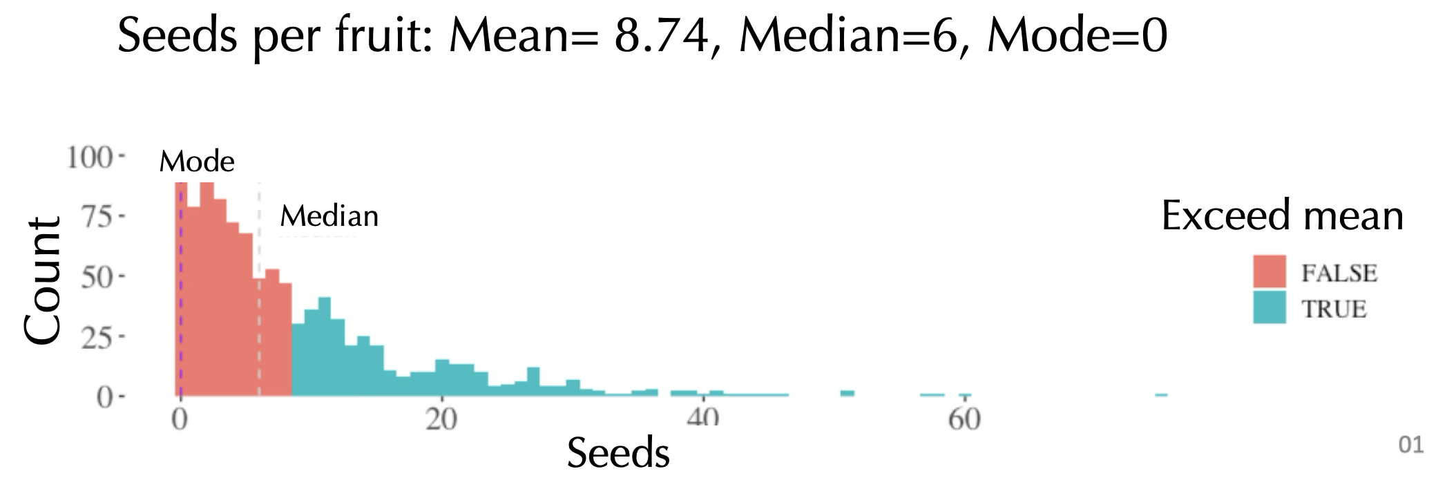
Mode

The most common value observed in a sample

• easy to pick out as the peak in a histogram

• Useful because it always reflects a value actually seen in the dataset, unlike mean and median

Mode

The most common value observed in a sample

• Unimodal vs bimodal (multimodal)

• Multimodal data usually reflects data has multiple (at least two) values that are equally common.

• Often results from two or more underlying groups being measured together.

• Can be used with data that isn’t numeric

But how will you know how your data is distributed?

First step: plot your data

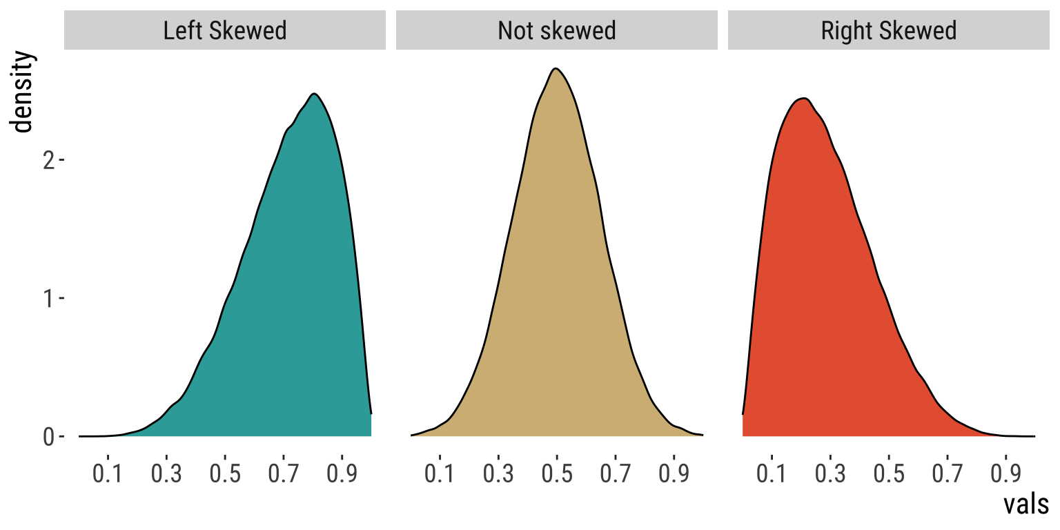
Skewness

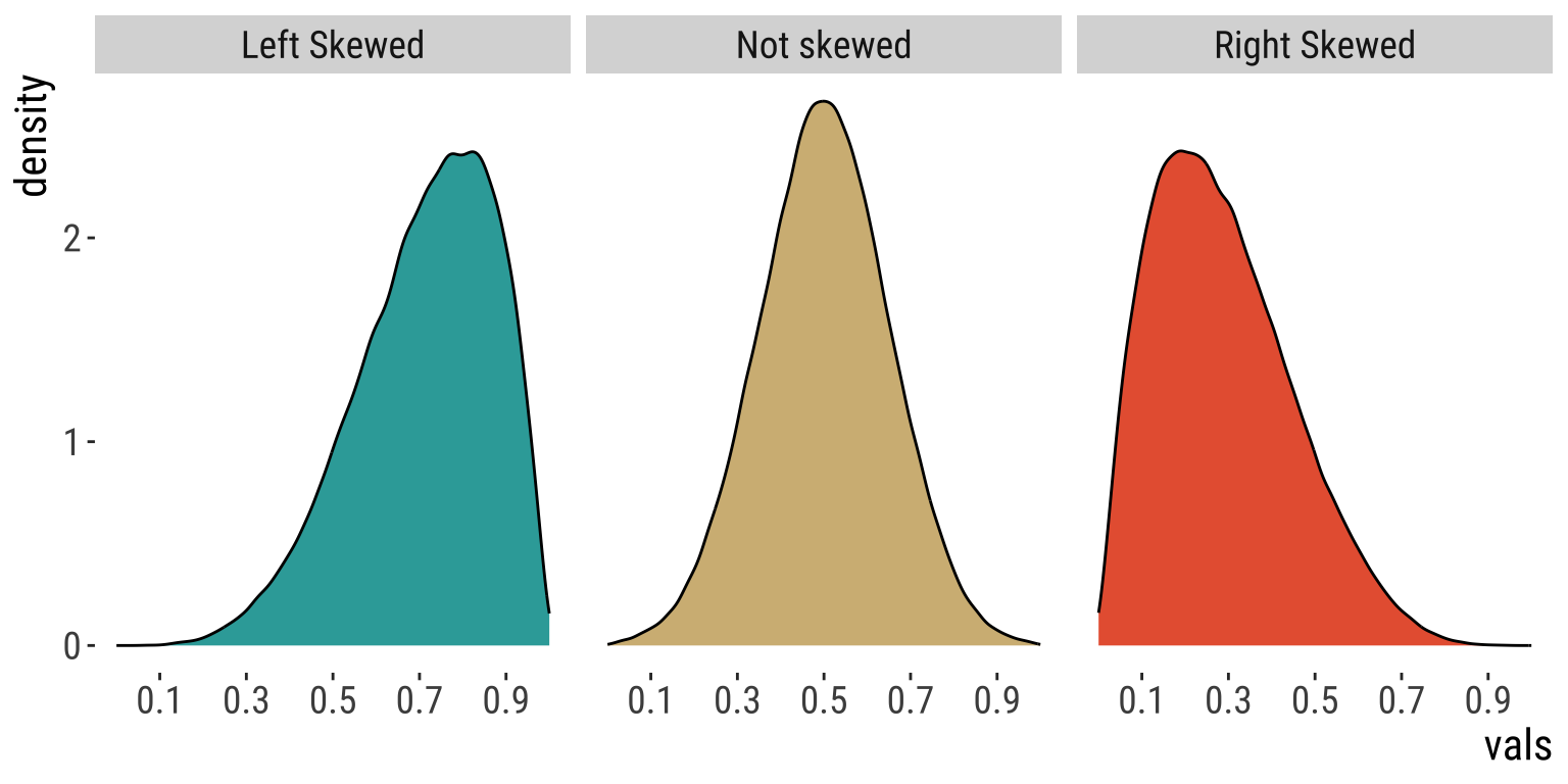
Skewness

Left: Asymmetric Few small values. \(>1/2\) of values exceed the mean.

Middle: Symmetric As many large as small values. \(\sim1/2\) of values exceed the mean.

Right: Asymmetric Few large values. \(>1/2\) of values are less than the mean.

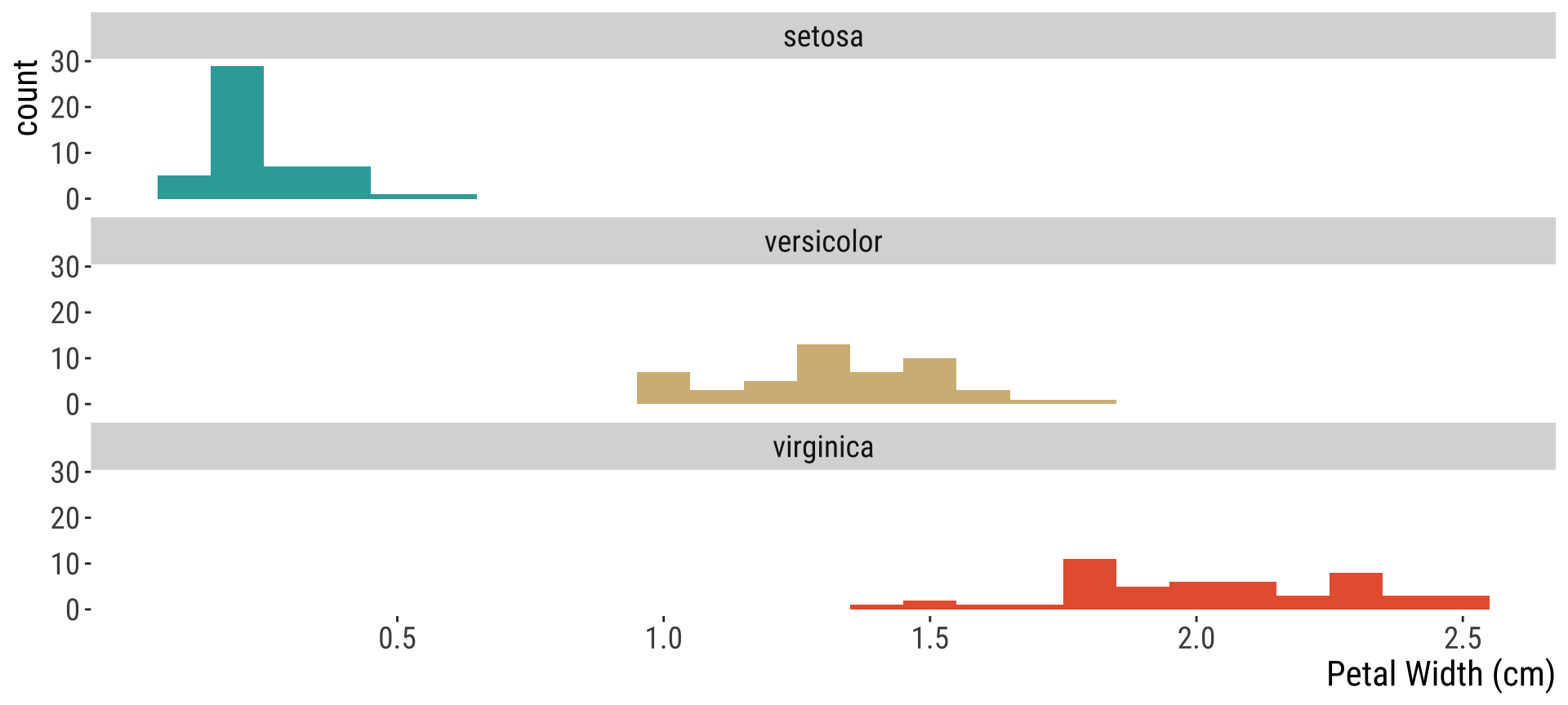
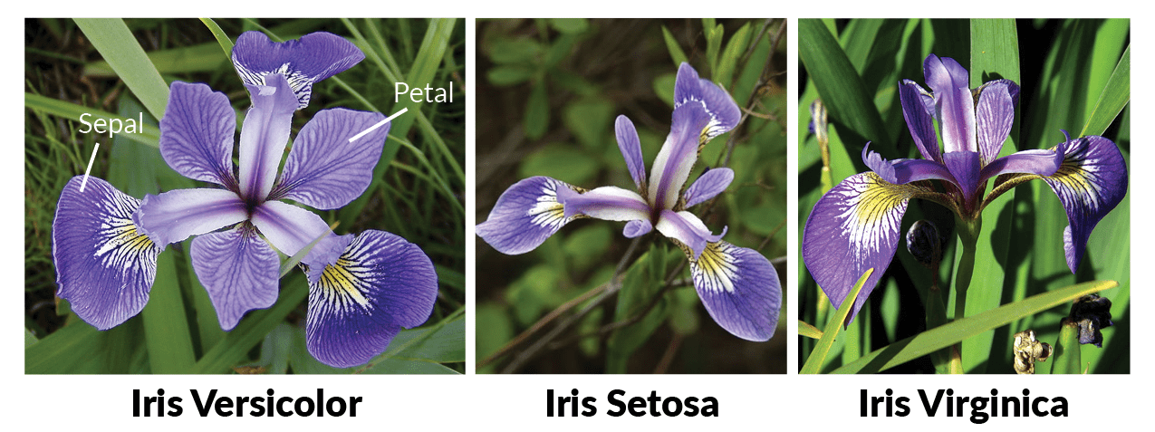
Histograms reveal measures of center

Recall the iris dataset

Histograms reveal measures of center

• Figure
• Code

library(ggplot2)
ggplot(iris, aes(x = Petal.Width, fill = Species)) +
    geom_histogram(binwidth = 0.1, show.legend = FALSE,
        alpha = 0.9) + xlab("Petal Width (cm)") + facet_wrap(~Species,
    ncol = 1) + scale_x_continuous(breaks = seq(0.5,
    2.5, 0.5)) + scale_fill_manual(values = wesanderson::wes_palette("AsteroidCity1")) +
    bb_theme()

Measures of dispersion

• Range [max value - min value]

• Quartiles, interquartile range [75th percentile - 25th percentile]

• Variance [ estimate = \(s^2\) =\(\frac{\Sigma(x_i - \bar{x})^2}{n-1}\), param = \(\sigma ^2\) = \(\frac{\Sigma(x_i - \mu)^2}{n}\) ]

• Standard deviation [ estimate = \(s\) =\(\sqrt{s^2}\), param = \(\sigma\) = \(\sqrt{\sigma^2}\) ]

• Coefficient of variation [ estimate = CV = \(\frac{s}{\bar{Y}}\), param = \(\frac{\sigma}{\mu}\) ]

Range

The difference between the maximum and minimum observed values in a sample

Range

Range of weight of 46 chicks at 20 days since birth

data("ChickWeight")
chick20 <- ChickWeight[ChickWeight$Time == 20, ]$weight
chick20

Max and Min in this dataset at time 20:

summary(chick20)

   Min. 1st Qu.  Median    Mean 3rd Qu.    Max. 
   76.0   161.0   204.0   209.7   259.0   361.0 

# or
c(min(chick20), max(chick20))

[1]  76 361

# commonly the diff between them is shown
max(chick20) - min(chick20)

[1] 285

That’s all for today

From: makeameme.org