2.3.Displaying & Describing Data

Measures of spread and plots

Bárbara D. Bitarello

2025-09-22

Last time

• Mean, median, mode
• Range

today: location and width; next class plots

This week

• Estimates of width (cont.)
• Explanatory and exploratory figures
• Best practices in figure design
• How data types drive figure design
• How to make effective tables

Recall this histogram

• Figure
• Mean and Median

# A tibble: 3 × 3
  Species     mean median
  <fct>      <dbl>  <dbl>
1 setosa     0.246    0.2
2 versicolor 1.33     1.3
3 virginica  2.03     2  

Measures of dispersion

• Range [max value - min value] (cont.)

• Quartiles, interquartile range [75th percentile - 25th percentile]

• Variance [ estimate = \(s^2\) =\(\frac{\Sigma(x_i - \bar{x})^2}{n-1}\), param = \(\sigma ^2\) = \(\frac{\Sigma(x_i - \mu)^2}{N}\) ]

• Standard deviation [ estimate = \(s\) =\(\sqrt{s^2}\), param = \(\sigma\) = \(\sqrt{\sigma^2}\) ]

• Coefficient of variation [ estimate = CV = \(\frac{s}{\bar{Y}}\), param = \(\frac{\sigma}{\mu}\) ]

Width (aka variability)

Variability of a population should not be ignored as simply noise about the mean, but is biologically important in its own right.

Variation has a true value from a population that we estimate from a sample.

Range

Range of weight of 46 chicks at 20 days since birth

data("ChickWeight")
chick20 <- ChickWeight[ChickWeight$Time == 20, ]$weight
chick20

Max and Min in this dataset at time 20:

summary(chick20)

   Min. 1st Qu.  Median    Mean 3rd Qu.    Max. 
   76.0   161.0   204.0   209.7   259.0   361.0 

# or
c(min(chick20), max(chick20))

[1]  76 361

# commonly the diff between them is shown
max(chick20) - min(chick20)

[1] 285

Range

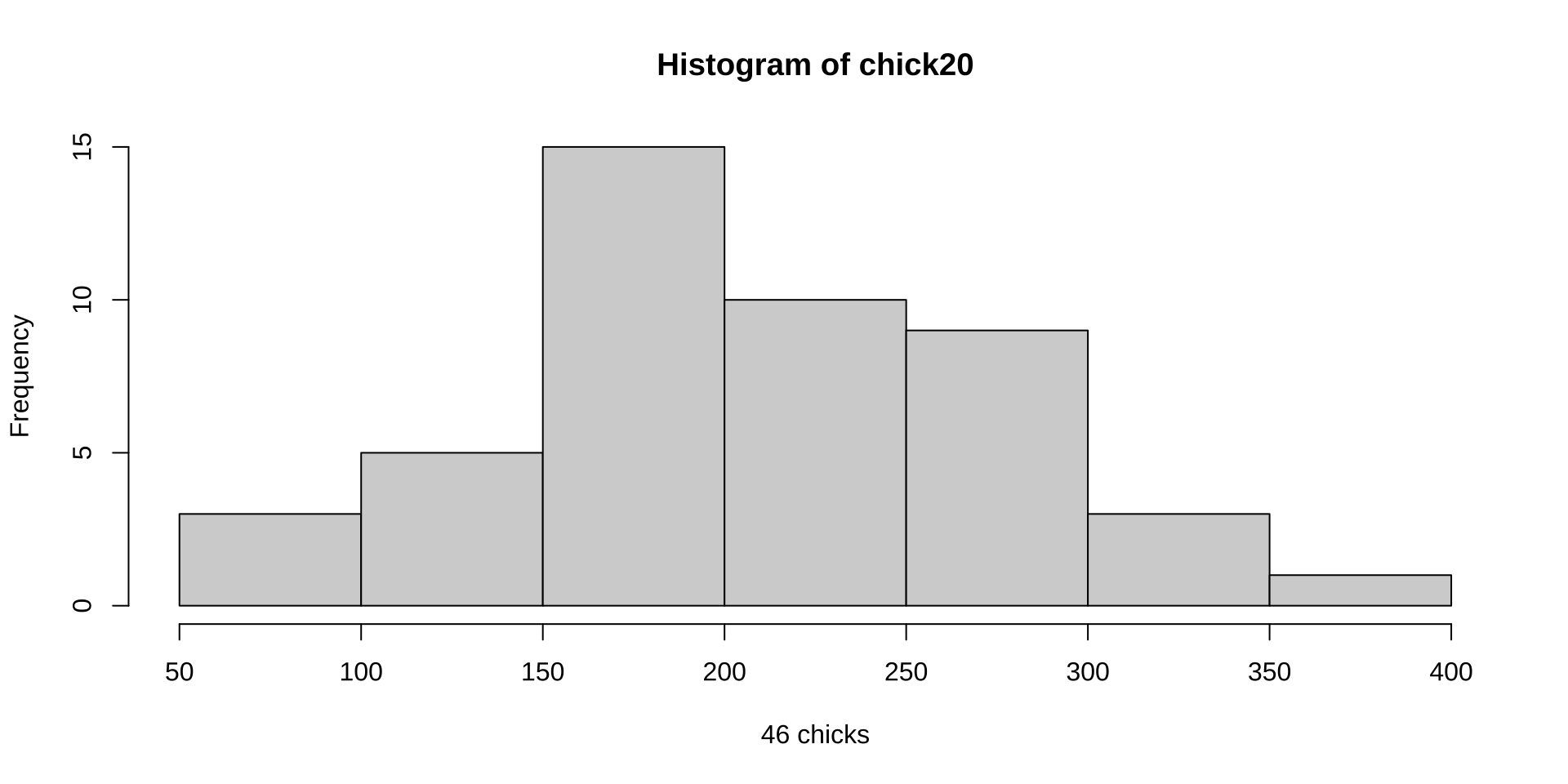
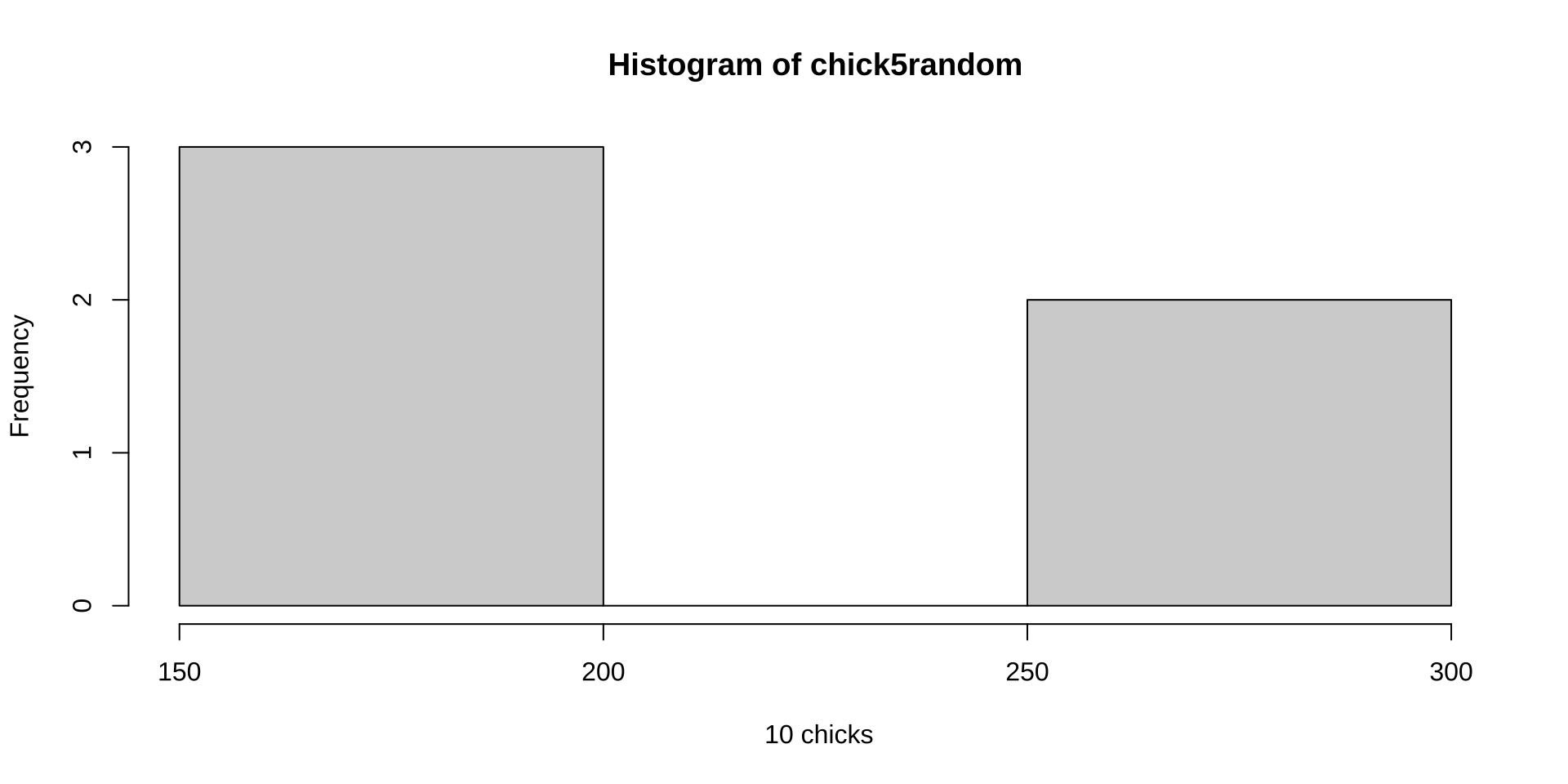
If I take a sample of just 5 chicks from those 46 …

range(chick20)

[1]  76 361

hist(chick20, xlab = "46 chicks")

chick5random <- sample(x = chick20,
    size = 5, replace = F)
range(chick5random)

[1] 157 295

hist(chick5random, xlab = " 10 chicks")

Small samples tend to give lower estimates of the range than large samples

So the sample range is a biased estimator of the true range of the population

So sample range is a biased estimator of the true range of the population.

Scenario

Salary range in a company will give a very good sense of the disparities between the ones in each end, but not a good sense of what the “average” employee earns

What can you do then?

You could calculate the median, sure, but what about the spread? Interquartile range would be a better measure here

Interquartile Range (IQR)

The difference between the 75th and 25th percentiles of the data. A.k.a., the “middle 50%” of the data.

• less biased estimator than range
• necessary for making boxplots

How?

IQR

Imagine sorting your data.

• The individual in the middle is the median.
• The first and last individuals mark the range
• The other two quantiles are the individuals ¼ and ¾ the way into your sorted list of data
• The difference between these is the interquartile range

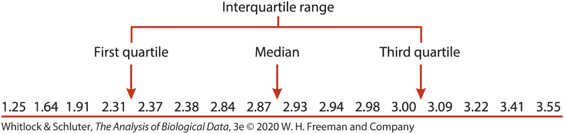
IQR Example

Example: Running speeds (cm/s) of Tidarren spiders before voluntary amputation of pedipalp

Attention:

• Quantiles partition the data into \(n\) parts
• Quartiles partition the data into quarters

IQR Example

\(n=16\)

1st quartile: \(j=0.25n=4\)

3rd quartile: \(j=0.75n=12\)

If \(j\) is integer, \(\frac{Y_{j}+Y_{j+1}}{2}\)

\(\frac{Y_{4}+Y_{5}}{2}=\frac{2.31+2.37}{2}=2.34\)

\(\frac{Y_{12}+Y_{13}}{2}=\frac{3+3.09}{2}=3.045\)

Note: software may use slightly different algorithms.

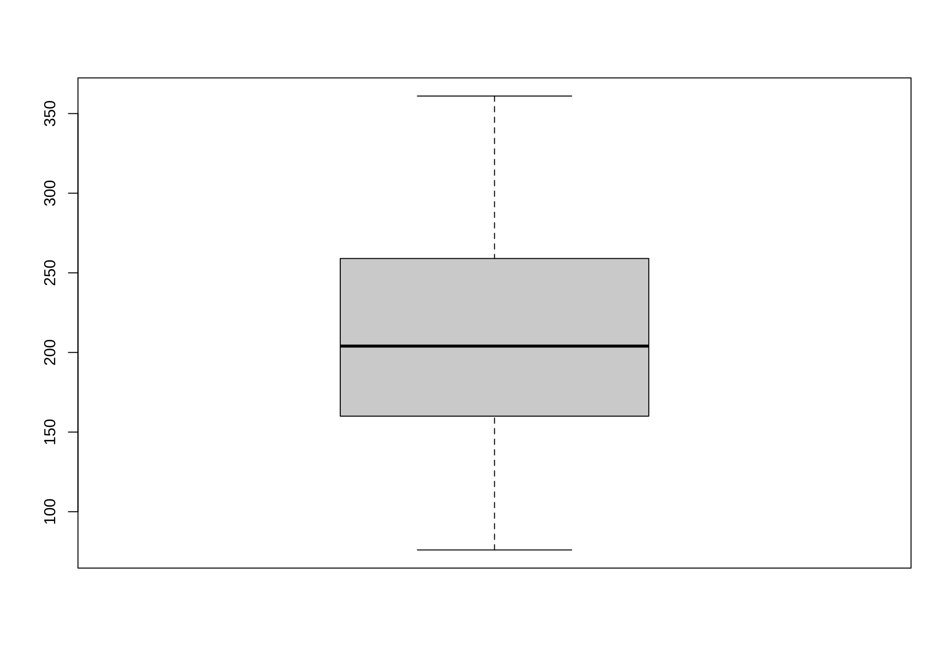
IQR in R

summary() gives quartiles and max/min

# summary gives quartiles and max/min
summary(chick20)

   Min. 1st Qu.  Median    Mean 3rd Qu.    Max. 
   76.0   161.0   204.0   209.7   259.0   361.0 

The “long” route:

as.numeric(summary(chick20)[5] - summary(chick20)[2])

[1] 98

The shortcut

IQR(chick20)

[1] 98

Boxplots reveal quartiles

boxplot(chick20, names = "chicks day 20")

IQR can give us more information than the range, but it’s still only looking at the values “in the middle”

But there are metrics that look at all the values

Variance, Standard Deviation, & Coefficient of Variation all communicate how far individual observations are expected to deviate from the mean.

Because (by definition) the differences between all observations and the mean sum to zero (\(\sum{Y_i-\bar{Y}=0}\)), these summaries work from the squared difference between observations and the mean (\(\sum{(Y_i-\bar{Y})^2}\)).

Variance

Variance is a measure of dispersion of data points in a sample (or population) around the mean of the sample (or population). It is the expected squared difference between an observations and the mean.

Variance

Parameter

\[\sigma^2=\frac{\sum_{i=1}^{N}(Y_{i}-\mu)^2}{N}\] \(N\): number of individuals in population

\(\mu\): population mean

Estimate

\[s^2=\frac{\sum_{i=1}^{n}(Y_{i}-\bar{Y})^2}{n-1}\] \(n\): number of individuals in sample

\(\bar{Y}\): sample mean

Note: the numerator here is called “sum of squares”

Sample variance (shortcut)

\[s^2=\left(\frac{n}{n-1}\right)\left(\frac{\sum^{n}_{i=1}{Y^2_i}}{n}-\bar{Y}^2\right)\]

Variance Example

Lifespan of 12 forager bees (in hours).

• Mean
• Sum of squares
• Sum of squares (cont)

2.3 2.3 3.9 4.0 7.1 9.5 9.6 10.8 12.8 13.6 14.6 18.2 18.2 19.0 20.9 24.3 25.8 25.9 26.5 27.1 30.0 33.3 34.8 34.8 35.7 36.9 41.3 44.2 54.2 55.8 65.8 71.1 84.7

\[\bar{Y} = \frac{\sum{Y_i}}{n} = \frac{919}{33}= 27.848\text{ hours}\]

beesDF |>
    mutate(`Y-meanY` = hours - mean(hours)) |>
    mutate(`(Y-meanY)^2` = (hours - mean(hours))^2)

# A tibble: 33 × 3
   hours `Y-meanY` `(Y-meanY)^2`
   <dbl>     <dbl>         <dbl>
 1   2.3     -25.5          653.
 2   2.3     -25.5          653.
 3   3.9     -23.9          574.
 4   4       -23.8          569.
 5   7.1     -20.7          430.
 6   9.5     -18.3          337.
 7   9.6     -18.2          333.
 8  10.8     -17.0          291.
 9  12.8     -15.0          226.
10  13.6     -14.2          203.
# ℹ 23 more rows

beesDF <- beesDF |>
    mutate(`Y-meanY` = hours - mean(hours)) |>
    mutate(`(Y-meanY)^2` = (hours - mean(hours))^2)
sum(beesDF[, 3])

[1] 13520.96

So

\[s^2 = \frac{13520.96}{33-1}=422.53\text{ hours}^2\]

Note: the unit here is hours squared. Also, note that we don’t divide by \(n\) but by \(n-1\).

4 differences from population mean:
s^2 instead of sigma^2; uses sample size instead of population size, taken as deviations from sample mean rather than population mean (which is not available); n-1, to account for bias caused by using Ybar (which is slightly closer to the individuals in the sample than the true mean is, because the sample mean is calculated from the sample too

Standard Deviation

Parameter

\[\sigma=\sqrt{\frac{\sum_{i=1}^{N}(Y_{i}-\mu)^2}{N}}=\sqrt{\sigma^2}\] \(N\): number of individuals in population

\(\mu\): population mean

Estimate

\[s=\sqrt{\frac{\sum_{i=1}^{n}(Y_{i}-\bar{Y})^2}{n-1}}=\sqrt{s^2}\] \(n\): number of individuals in sample

\(\bar{Y}\): sample mean

Standard Deviation

Using the previous example, with forager bees.

\[s^2 = \frac{13520.96}{33-1}=422.53\text{ hours}^2\] \[s = \sqrt{422.53}=20.555\] ## In R

Variance

var(beesDF$hours)

[1] 422.5301

Standard deviation

sd(beesDF$hours)

[1] 20.55554

sqrt(var(beesDF$hours))

[1] 20.55554

Coefficient of Variation (CV)

• The variance and standard deviation increase with the mean.

• The coefficient of variation allows for fair comparisons of variability between measures on different scales.

\[CV = 100\% \times \frac{s}{\bar{Y}}\]

In summary

Range: The difference between the largest and smallest values.

Interquartile Range: The difference between the 25th and 75th percentile.

Variance & Standard Deviation: The difference between observations & the mean.

Coefficient of Variation: A measure of the standard deviation that’s independent of the mean.

Variance, Standard Deviation or Coefficient of Variation?

Variance and standard deviation convey the same information and are used in many equations.

The coefficient of variation is less directly used in equations, but is ideal for comparing variation between different types of comparisons.

That’s all for today

From: makeameme.org