4.3.Estimation with Uncertainty
2025-10-29
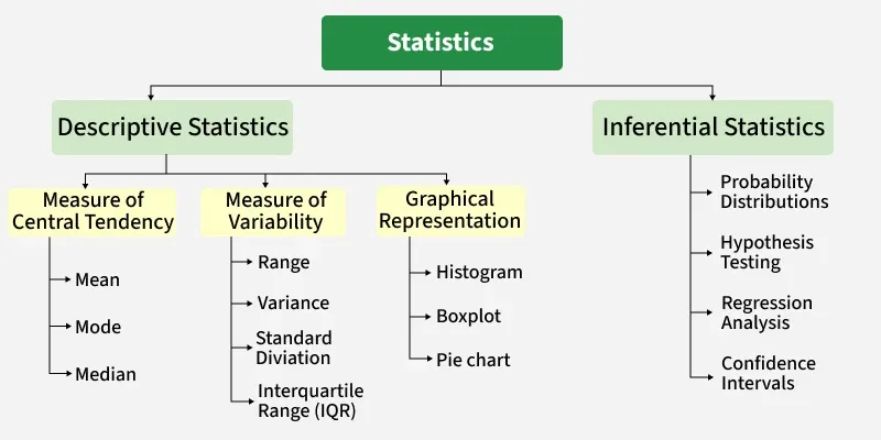
Inferential Statistics
The sampling distribution is at the heart of statistics
Q: But why do we need the sampling distribution?
A:
The Sampling Distribution
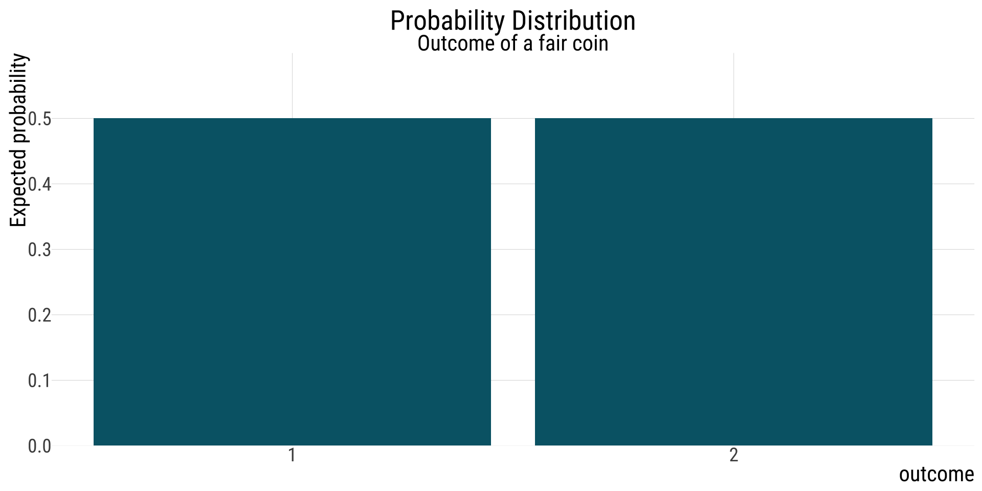
Let’s start from the very beginning. Consider the roll of a six-sided die.
This probability distribution shows all possible outcomes of a single die roll and how likely they are. I.e., in the long term, if you roll the die MANY times, you would expect equal proportions of each result.
What about a streak?

The sampling distribution can help us here.
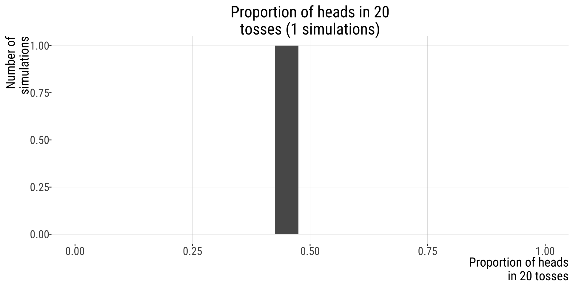
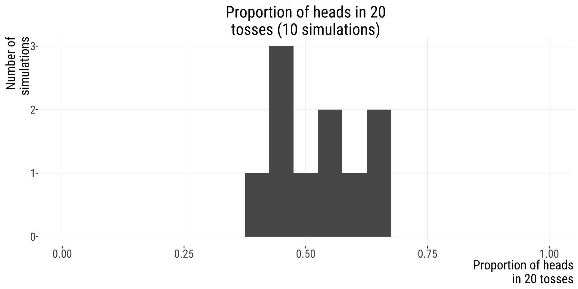
Example: possible outcomes of tossing a fair coin 20 times
One possible outcome leads to this histogram:
Repeat this process 10 times
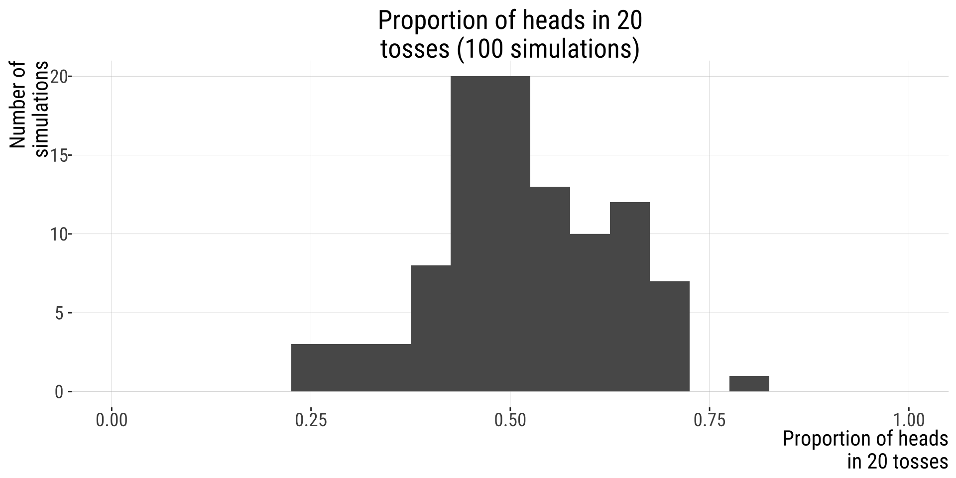
100 times
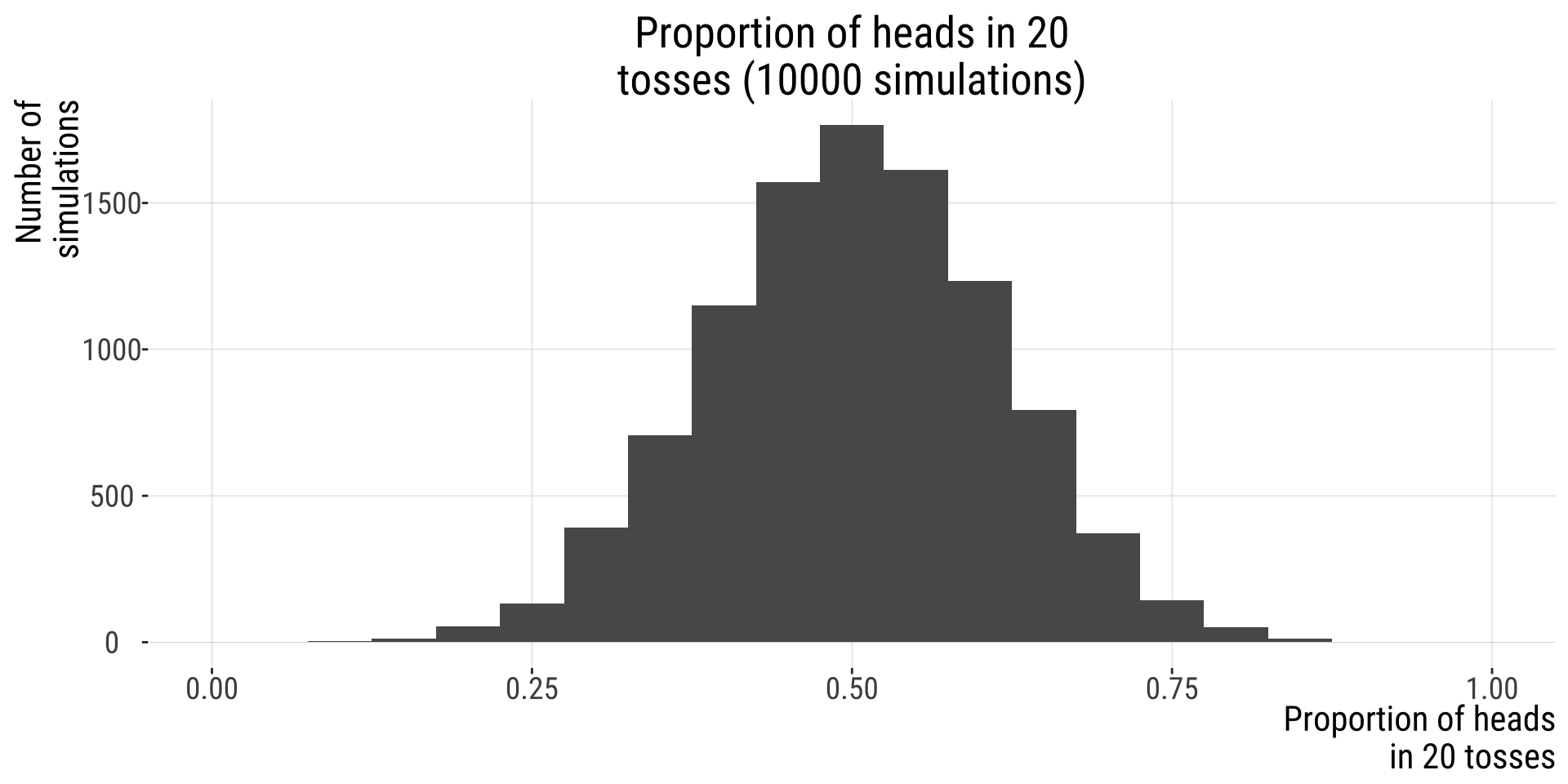
10000
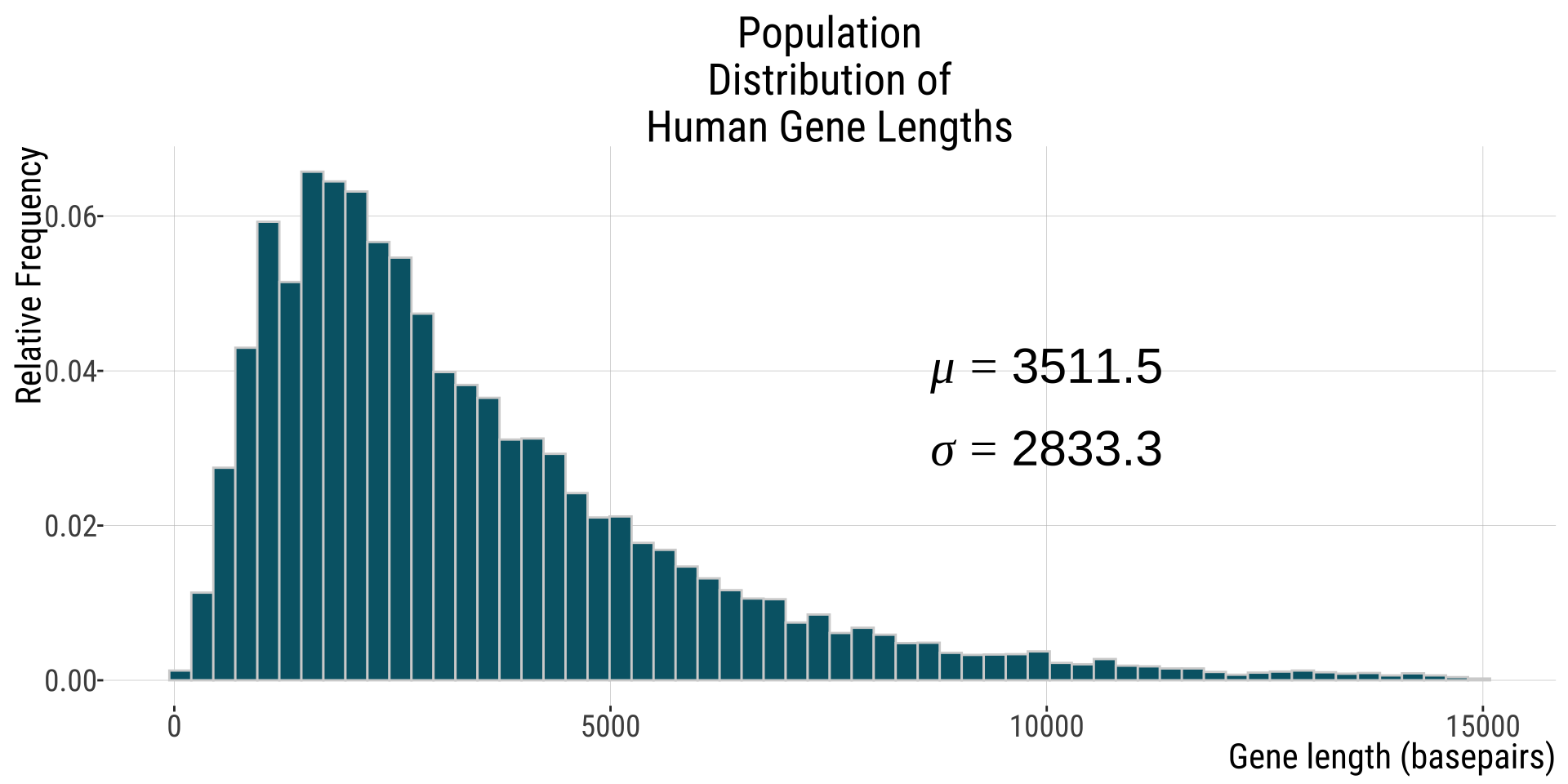
Population distribution
In our previous example, we were interested in the lengths of human genes.
- Population distribution: contains all values (all human gene lengths). Here is the histogram
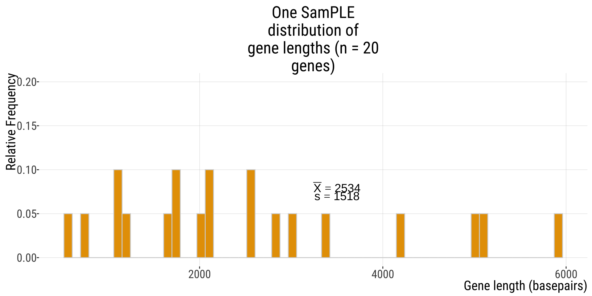
SamPLE distribution of gene lengths
Say, from one sample of 20 genes.
- the samPLE distribution will be based on the individual values of the individuals from my sample (in this case, 20 genes, sampled without replacement)
Another 20 genes sample
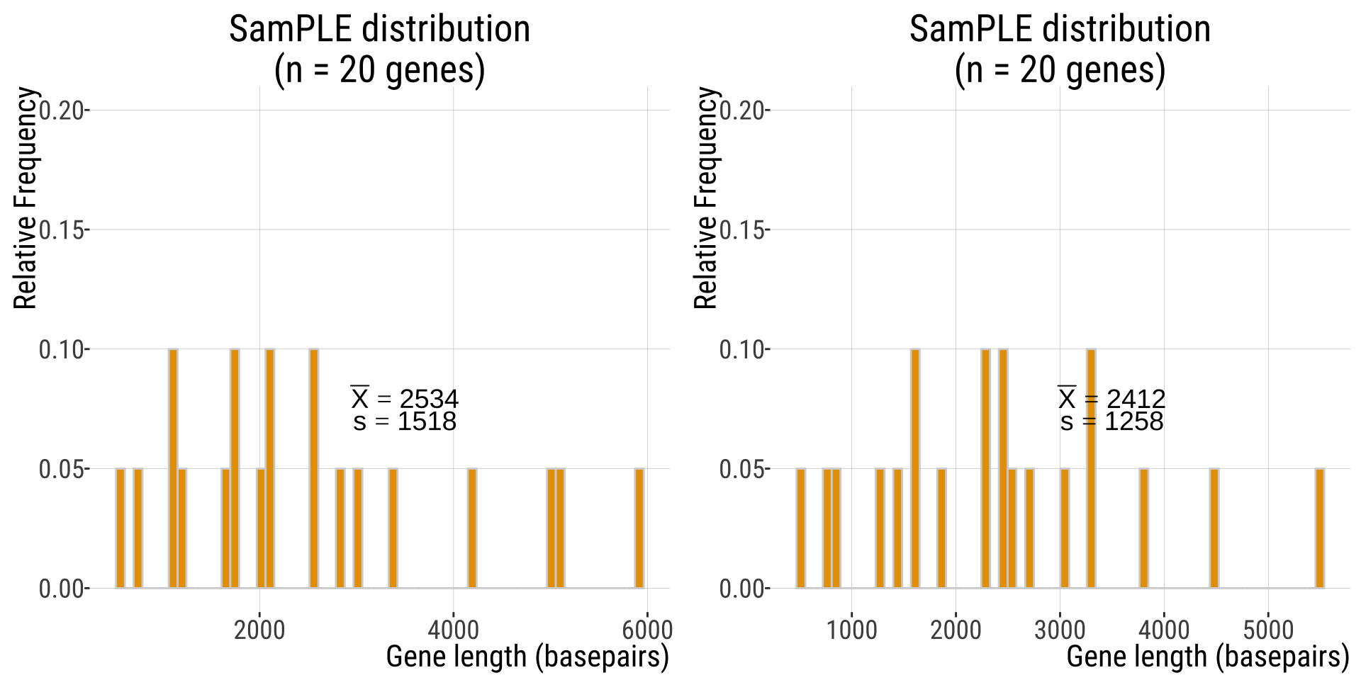
Another
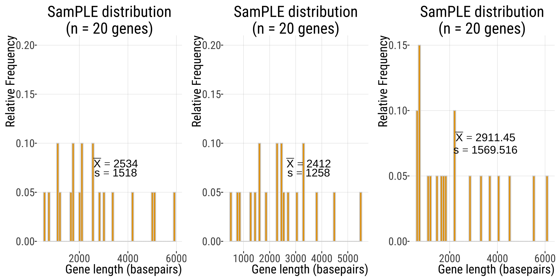
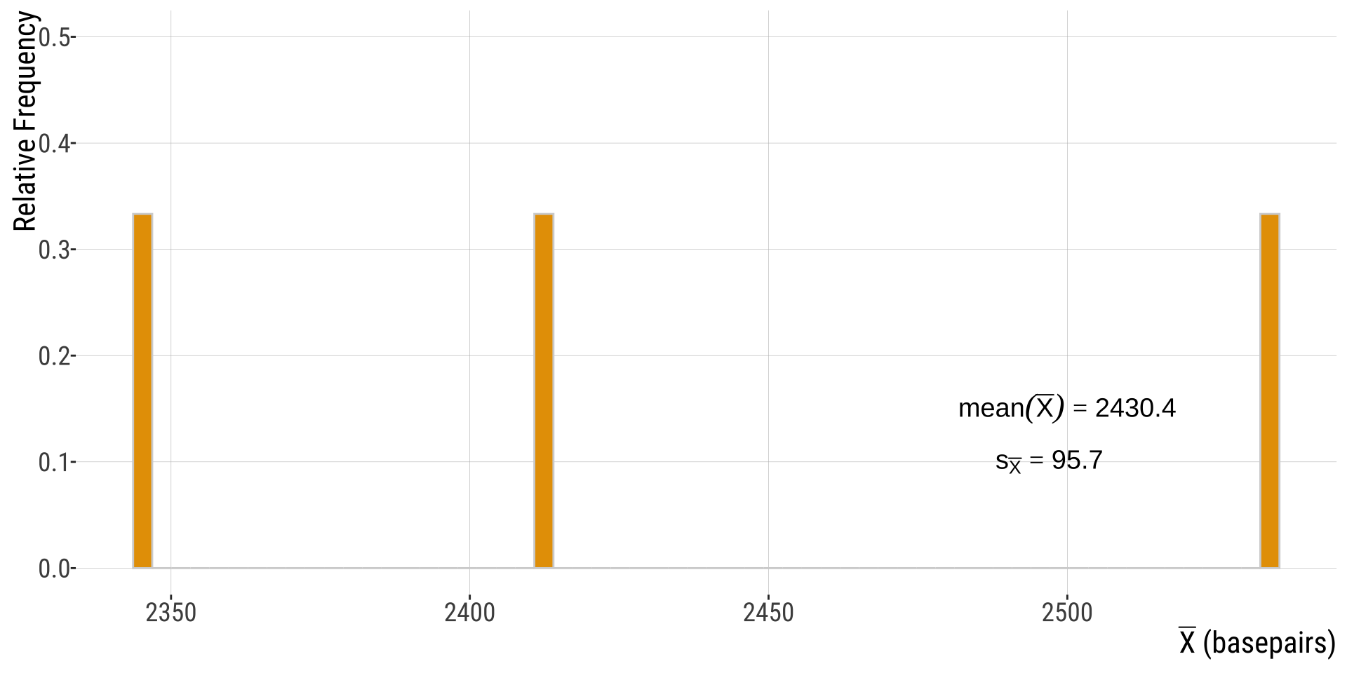
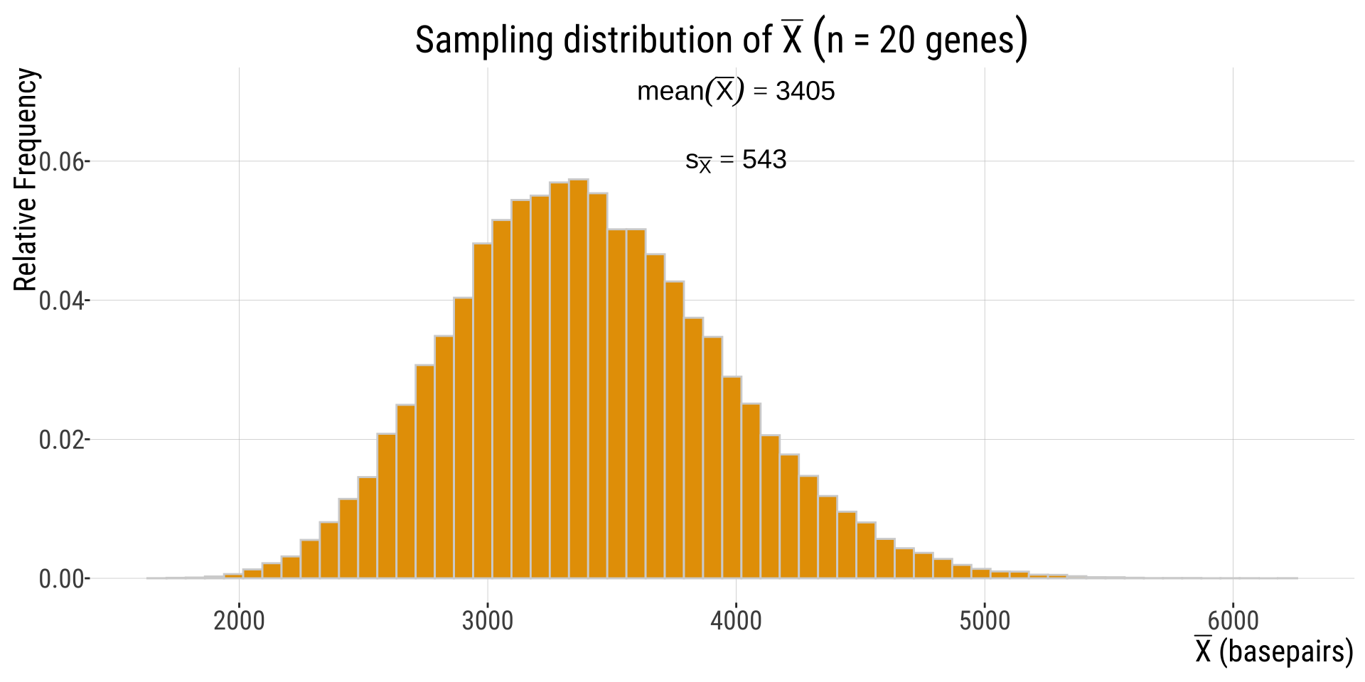
SampLING distribution
In this case, the samplING distribution of mean gene lengths.
We can start building this by collecting the individual samPLE means we calculated before: \(\bar{X}=\{3110.3,2412,2911.45,...\}\), and making a histogram of \(\bar{X}\)s.
Increasing number of repetitions…
If instead of taking 3 independent samples of 20 genes we take, say, 100,000, we see a sampling distribution
Compare
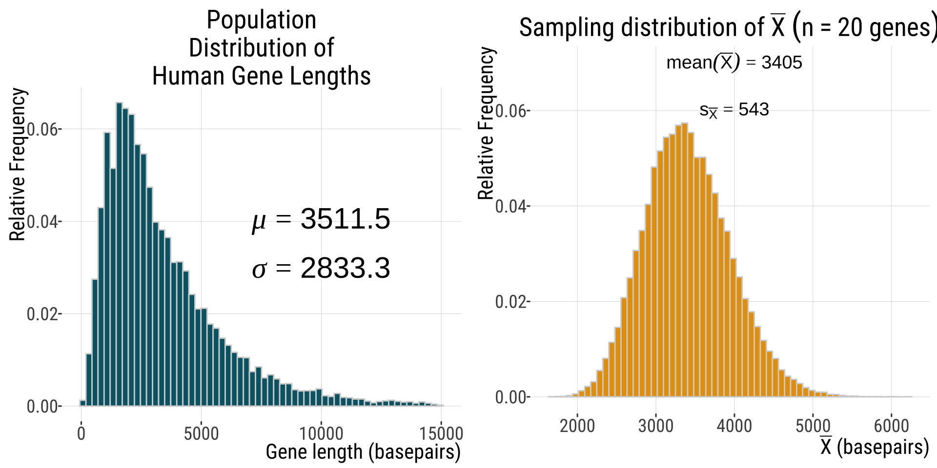
Grand mean of \(\bar{X}\) approaches population mean \(\mu\)
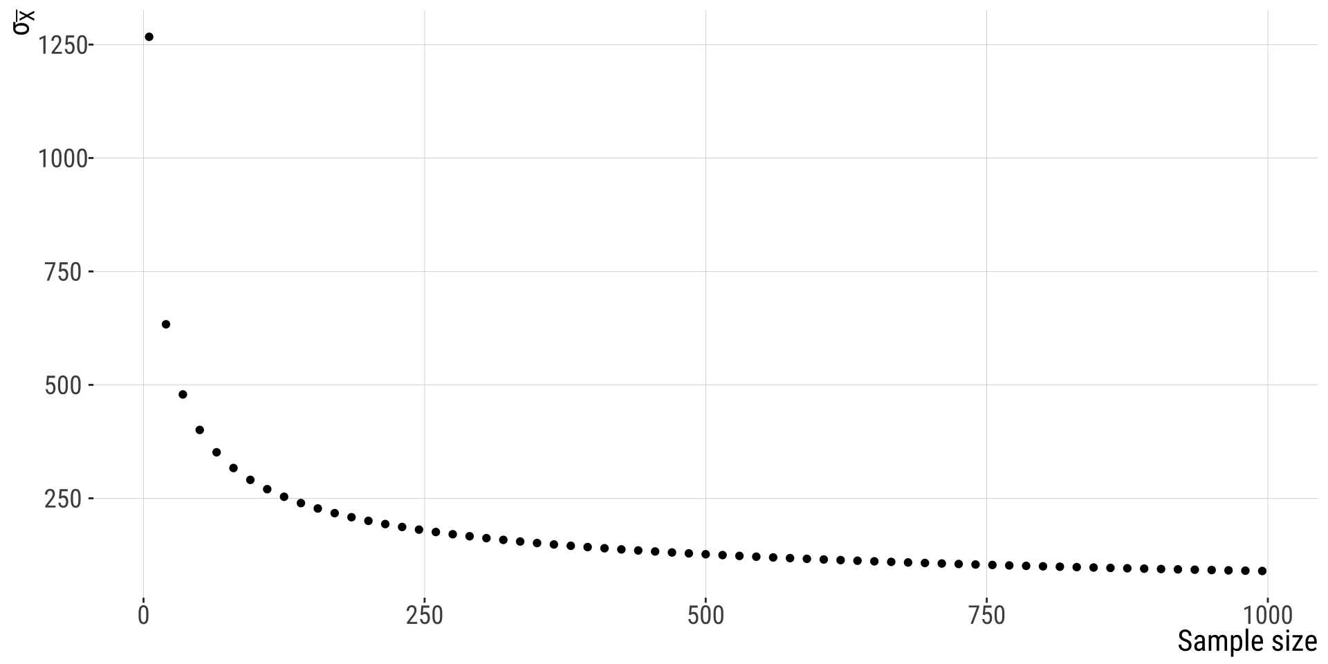
SE Decreases with Sample Size
That’s all for today

From: makeameme.org