Key learning goals
- Be able to describe the Null Hypothesis.
- Understand the practice of Null Hypothesis Significance Testing.
- Master the meaning of a P-value.
- Have the basis to be critical and skeptical of P-values.
- Explain the concepts of false positives and false negatives and why they happen.
- Understand when to use one vs two-tailed tests.
- Understand the relationship between p-values and CIs
Outline
- Estimating p-value and interpreting it
- Cautionary tales
- Type I and type II errors in hypothesis testing
- Estimation vs. hypothesis testing
- Philosophical/historical digression/discussion about p-values (optional readings posted in course website)
Recap Question 1
Which of the choices below is an appropriate alternative hypothesis for a null hypothesis which reads: “the mean systolic blood pressure for men is 120”?
A. The mean systolic blood pressure for men differs from 120.
B. The mean systolic blood pressure for men differs from that of women.
C. The mean systolic blood pressure for men is less than 120.
D. The mean systolic blood pressure for men is more than 120.
Recap Question 2
The P-value is best described as the probability that
A. We would observe the data we do if the null hypothesis is false.
B. We would observe the data we do if the null hypothesis is true.
C. The null hypothesis is false.
D. The null hypothesis is true.
Recap: The Steps of Hypothesis Testing
State \(H_0\) and \(H_A\).
Calculate a test statistic.
Generate the null distribution.
Find critical value at specified \(\alpha\), and the p-value.
The P-value: a measure of surprise
![]()
The Scream, by Edvard Munch - National Museum of Art, Architecture and Design, Public Domain
P-value
The p-value is the probability a sample from the null model would be as or more extreme than our sample. It quantifies your surprise if you assumed that the null was true.
More formal definitions:
The strength of evidence in the data against the null hypothesis
The long-run frequency of getting the same result or one more extreme if the null hypothesis is true.
![]()
P-value
p-value = the probability of obtaining a test statistic at least as extreme as the one from the data at hand, assuming:
- the model assumptions for the inference procedure used are all true, and
- the null hypothesis is true, and
- the random variable is the same (including the same population), and
- the sample size is the same.
Notice that this is a conditional probability (\(P(\text{observed_effect}|\text{null hypothesis is true})\): The probability that something happens, given that various other conditions hold. One common misunderstanding is to neglect some or all of the conditions.
Finding P-values
Evaluating where the test statistic lies on a sampling distribution built from the null model.
We generate this null sampling distribution by:
Simulation
Permutation (shuffling)
Mathematical results developed by professional statisticians. These are built from the logic of probability theory.
Unremarkable P-value
We would not be surprised if the sample below came from the null model.
![]()
A remarkable P-value
We would be very surprised if the sample below came from the null model.
![]()
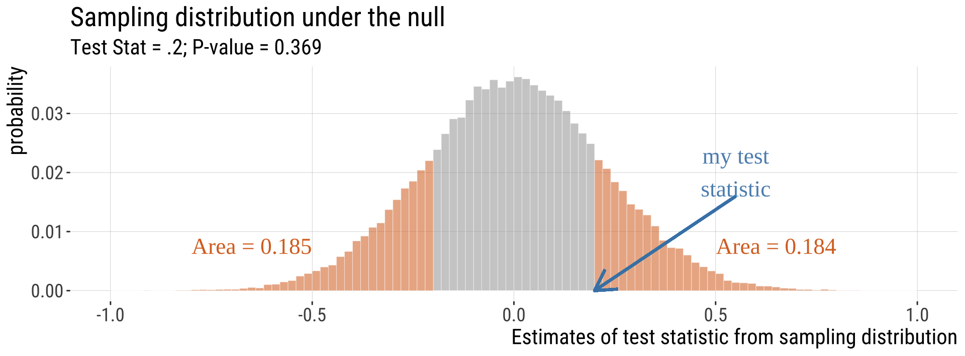
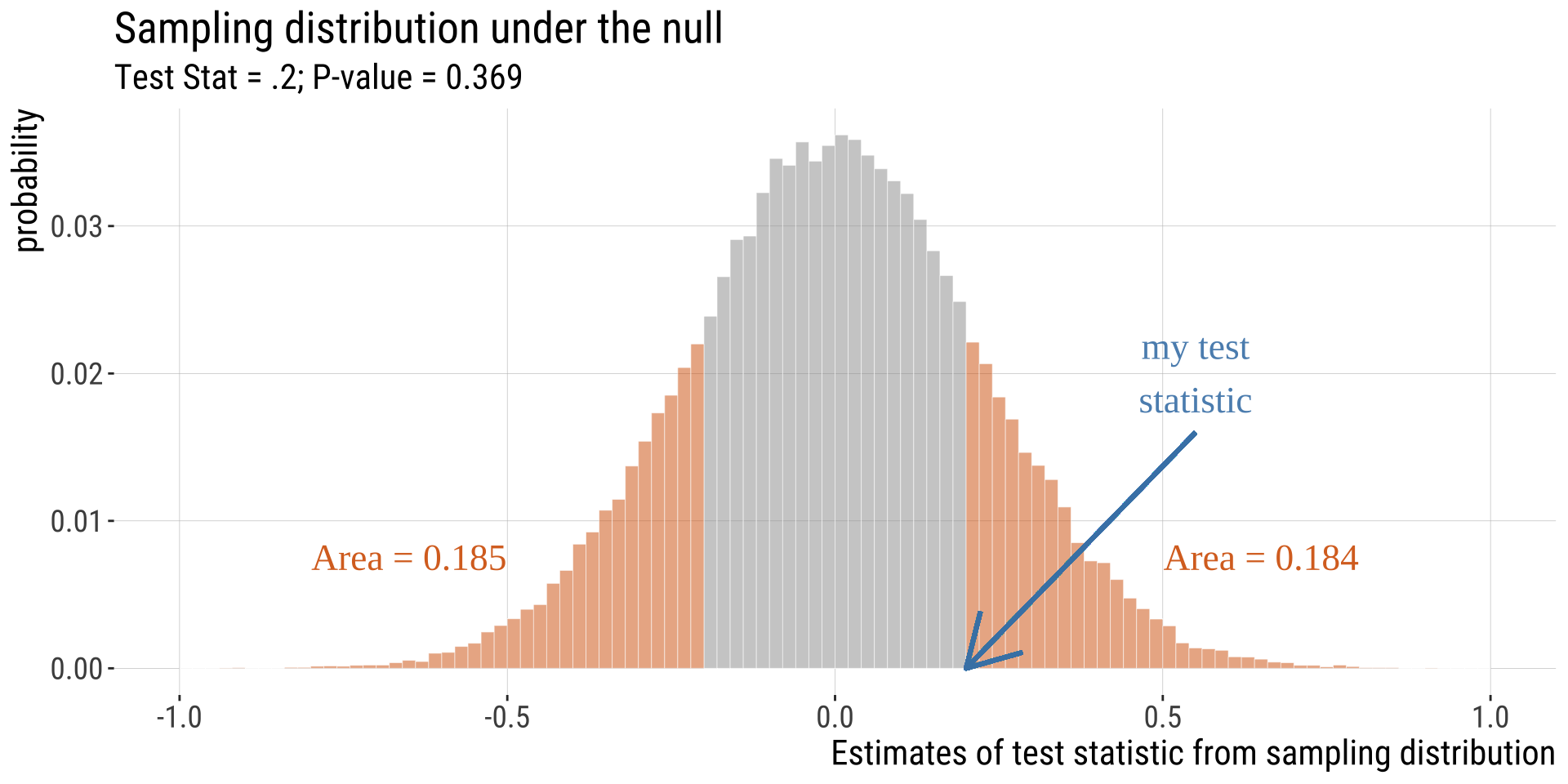
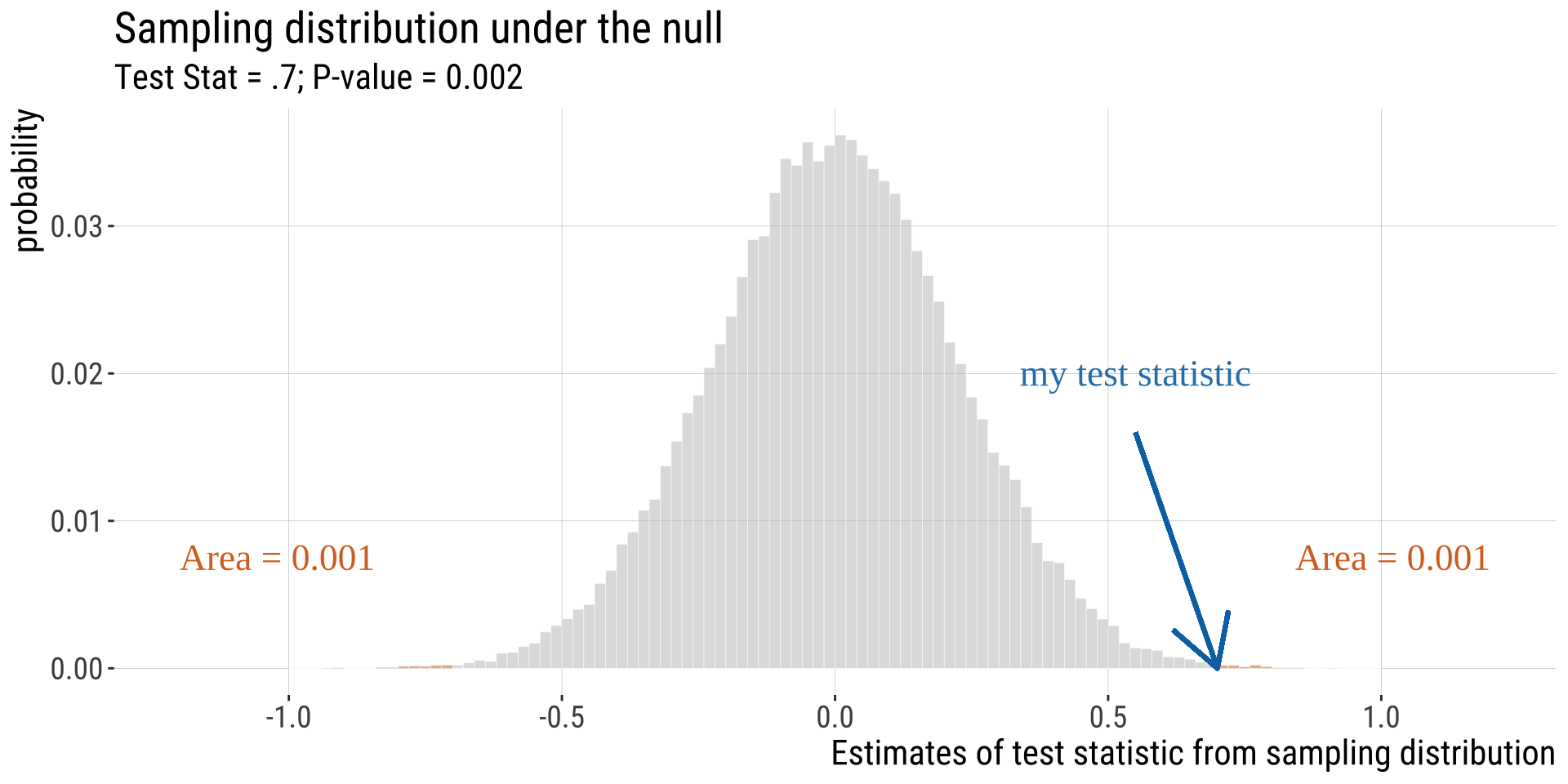
Most Tests Are Two-Tailed
- This means that a deviation in either tail of the distribution would be worth reporting.
![]()
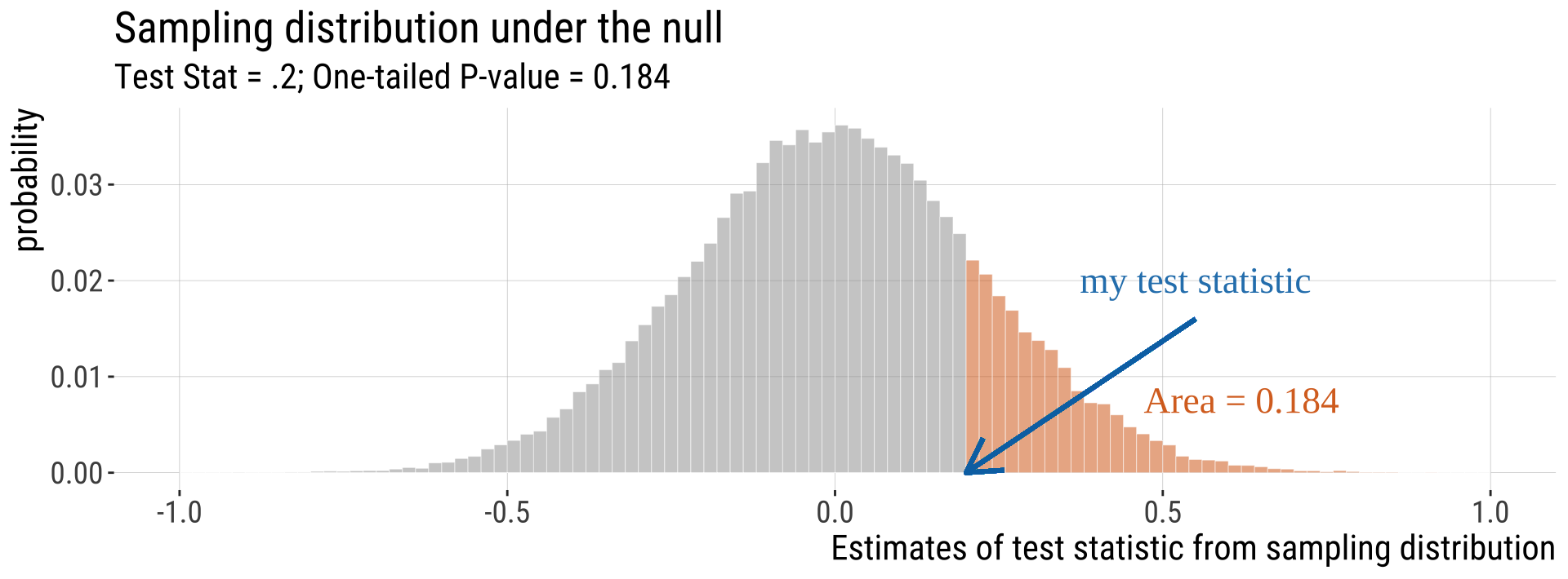
One-tailed P-values
- If a tail of the distribution is nonsense, calculate a P-value without it. We’ll see that \(\chi^2\) tests and F-tests are usually 1-tailed.
![]()
One vs two-tailed tests
One-tailed
- When planning a study, choosing a one-tailed P value gives you a more focused hypothesis and so reduces the necessary sample size.
- A study designed to use a one-tailed P value requires about 20% fewer subjects than the same study de-signed to use a two-tailed P value (Moyé & Tita, 2002). This reduces costs
- Once the data are collected, the appeal is clear: assuming you predicted the direction of the effect correctly, a one-tailed P value equals 1/2 of the two-tailed P value (not always true, but true for most statistical tests).
-
You should only report a one-tailed P value when you have predicted which treatment group will have the larger mean (or proportion, survival time, etc.) before you collect any data and have recorded this prediction (so you can’t be tempted to change your “prediction” after viewing the data)
One vs two-tailed tests
Two-tailed
- When in doubt, use a two-tailed P value
- The relationship between P values and CIs is more straightforward
- Some tests compare three or more groups, in which case the concept of one or two tails makes no sense.
- The practical effect of choosing a one-tailed P value is to make it appear that the evidence is stronger (because the P value is lower). But this is not due to any data collected in the experiment, but rather to a choice (or perhaps a belief) of the experimenter.
- Some reviewers or editors may criticize any use of a one-tailed P value, no matter how well you justify it. ::: aside Credit: This slide uses materials from the textbook Intuitive Biostatistics, Motulsky, 4th edition :::
A Guide To P-values From
The ASA
P-values can indicate how incompatible the data are with a specified statistical model (aka, the null hypothesis).
P-values DO NOT measure the probability that the studied hypothesis is true, NOR the probability that the data were produced by random chance alone.
P-values DO NOT measure the size of an effect or the importance of a result. (you can have small effects and very significant p-values and vice-versa)
Scientific conclusions & business or policy decisions should not be based only on whether a P-value passes a specific threshold.
A p-value, or statistical significance, does not measure the size of an effect or the importance of a result.
By itself, a p-value does not provide a good measure of evidence regarding a model or hypothesis.
Proper inference requires full reporting and transparency.
Statistical Significance and Making Binary Decisions
Statistical Significance
The significance level, \(\alpha\), is the probability used as the criterion for rejecting the null hypothesis.
The significance level \(\alpha\) is the probability of making the wrong decision when the null hypothesis is true.
If the P-value is \(\leq \alpha\), we reject the null hypothesis, and say the result is “statistically significant”
The value of the test statistic required to achieve \(P \leq \alpha\) is called the “critical value”
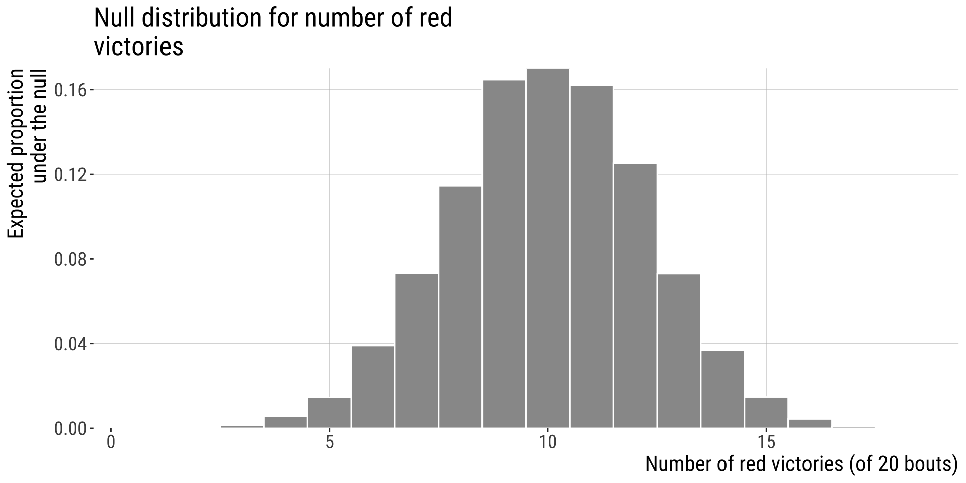
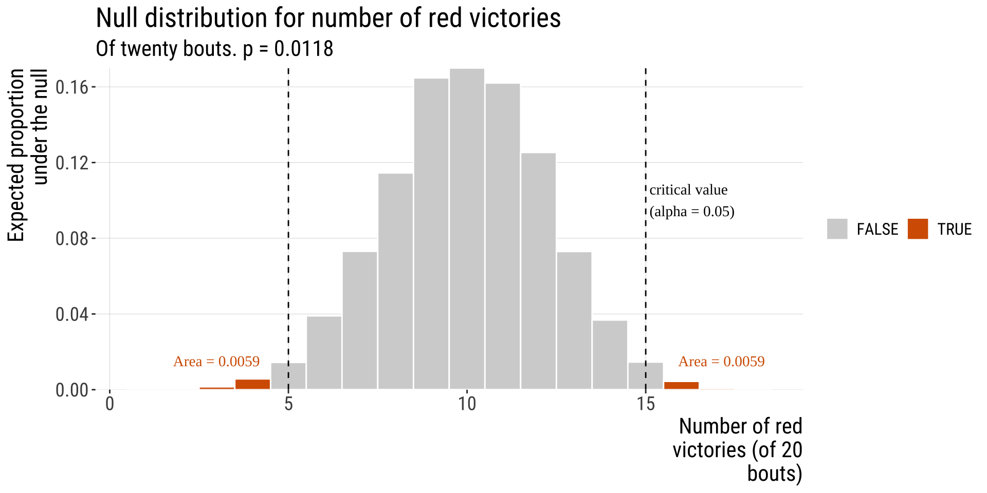
Wrestlers’ shirt color example
Step: 4-5: Find the critical Value & P-Value
- What is the probability of obtaining data as extreme or more extreme (in relation to the null distribution) than the one I obtained?
- Because finding the critical value depends on the sampling distribution, we will not go into it now but we will once we talk about specific tests. In this problem specifically the sampling distribution is the binomial and it has known properties.
Wrestlers’ shirt color example
Step: 4-5: Find the critical Value & P-Value
- In our example, we have 20 trials (rounds), and we expect victories to be equally distributed across shirt colors worn by wrestlers (\(p_{success}=0.5\)). We had 16 rounds won by red shirt-wearing wrestlers (\(\hat p=16/20 = 0.80\)):
Two tailed P-value: \(P(X \leq 4)+ P(X \geq 16)\)
\(=0.0059 + 0.0059 \approx 0.01182\)
Decide and conclude
\(P =\) 0.0118, so this result is unlikely under the null.
We reject \(H_0\) at the \(\alpha = 0.05\) significance threshold.
We conclude that red shirts perform better than we can reasonably expect by chance.
But we recognize that given many tries a pattern this extreme (or even more extreme) can occur without any dependence between victory and shorts color.
Hypothesis Testing: What Could Go Wrong?
Even if you do everything right, hypothesis testing can get it wrong.
Hypothesis testing can go wrong in two types of ways:
- Rejecting a true null (False positive or type I error, aka \(\alpha\)).
- Not rejecting a false null (False negative or type II error). Incorrectly concluding that there is no effect in the population when there truly is an effect.
Type I and type II errors are theoretical concepts. When you are analyzing a sample you don’t know whether you are making this kind of error or not. The only exception is when you’re simulating a scenario and checking the performance of a test on simulated data.
Statistical power
- A measure of the capacity of an experiment to find an effect (a ‘statistically significant result’) when there truly is an effect.
- The probability that a random sample will lead to rejection of a false null hypothesis.
- Very difficult to quantify - we usually don’t know how different the truth is from the null hypothesis.
What improves statistical power?
- Larger sample size
- The magnitude of the true discrepancy from the null hypothesis (aka the “effect size”)
- Low variability in the population of interest
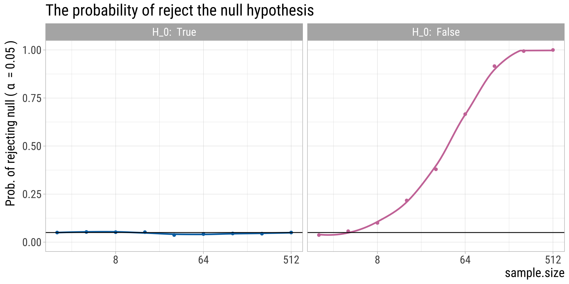
Effects of Sample Size
The exact relationship between several features of the experiment: the threshold for significance (\(\alpha\)), size of the expected effect, variation present in the population (variance), alternative hypothesis (one or two sided), nature of the test (paired or unpaired), and sample size.
![]()
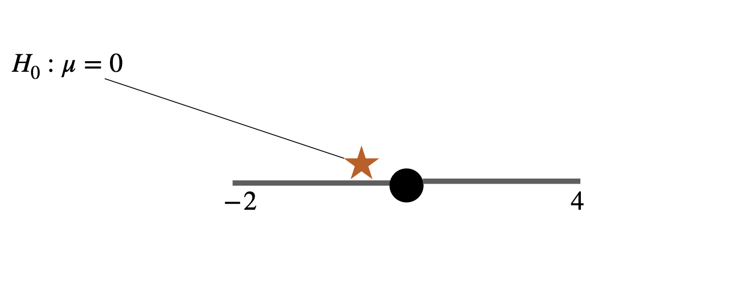
Hypothesis Testing vs. Confidence Intervals
“Imperfectly understood CIs are more useful and less dangerous than incorrectly understood P values.” – Hoenig and Heisey (2001) The abuse of power: the pervasive fallacy of power calculations for data analysis. The American Statistician, 55(1), 19-24.
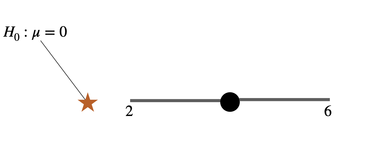
Would confidence intervals and hypothesis tests on the same data give same answer?
If the parameter value stated in the null hypothesis falls outside of the 95% confidence interval you estimated, it is almost certain your P-value will be significant at α = 0.05
![]()
If the parameter value stated in the null hypothesis falls inside of the 95% confidence interval you estimated, it is almost certain your P-value will be nonsignificant at α = 0.05
![]()
Why not ditch the P-value and hypothesis testing in general and just use the CI, then?
Estimation vs. Hypothesis Testing
Both use sample data to make inferences about the underlying population
CI
Estimation is quantitative: it quantifies, puts a bound on the likely values of a parameter, and gives me the size of the effect
More revealing about the magnitude of the parameter or treatment effects
Does everything hypothesis testing can do
And yet are way less used in biological research
Hypothesis Testing
Hypothesis testing is more qualitative: does the estimated parameter value differ from a null model? Is there any effect at all (yes or no)
Widely used in biology
Decide (yes/no) whether sufficient evidence has been presented to support a scientific claim
They work very well together. Providing P- values and point estimates + CI is currently the best way to go
Caveats and Cautionary Tails
Reminders
Correlation \(\neq\) causation
Confounding variables: an unmeasured variable that may cause both X and Y
-
Observations vs. Experiments:
Observed correlations are intriguing, and can generate plausible and important hypotheses.
Correlations in treatment (x) and outcome (y) in well-controlled experimental manipulations more strongly imply causation because we can (try to) control for confounding variables.
Statistical Significance
\(\neq\) Biological Importance
- High powered Genome Wide Association Studies (GWAS) often identify loci associated with negligible increases in the chance of acquiring some disease.
Significant? Important?
| Significant |
Polio vaccine reduces incidence of polio |
Things you don’t care about, or already well known things |
| Not Significant |
Suggestive evidence in a small study, leading to future work. OR No support for a thing thought to matter in a large study. |
Studies with small sample size and high P-value OR Things you don’t care about. |
Multiple testing
- If you perform several hypothesis tests within one study, there is a chance you will get at least one significant p-value.
- Methods exist to control for multiple testing for this reason.
- Most popular tool is called the Bonferroni correction
Example: astrology and health conditions
In a study, authors searched through a health database of 10 million residents of Ontario, Canada, collecting their reason for admission into a hospital and their astrological sign. They then asked if people with certain astrological signs are more likely to be admitted to the hospital for certain conditions
Result: 72 diseases occurred more frequently in people with one astrological sign than in people with all other astrological signs, and this different was found to be statistically significant
WOW!!!
…Wow, right?
- Their significant level going in was α = 0.05
- I.e., the null hypothesis is rejected if a result as or more extreme than the one observed occurs with p < 0.05
- Conclusion: there is a conniving relationship between astrological sign and health outcomes of individuals…right?
Not quite
- Problem: Austin et al. looked at 233 conditions and 12 astrological signs, meaning they did 233 × 12 = 2,796 different hypothesis tests in this study
- Therefore: they would expect to find a false positive in \(0.05 \times 2796 = 139.75\) times! In reality, they only found 72
- The result was not impressive at all!
- Note: this study was not an epic fail. It wasn’t looking at this relationship “for real” but rather the difficulty of interpreting statistical results.
Family-wise error rate
Whenever you perform a hypothesis test, there is a chance of committing a type I error (rejecting the null hypothesis when it is actually true).
For ONE hypothesis test: the type 1 error rate (false positive) is simply α–the significance level!
When we conduct multiple hypothesis tests at once, we have to deal with something known as a family-wise error rate, which is the probability that at least one of the tests produces a false positive:
\[\text{Family-wise error rate}= 1-(1-\alpha)^n\] \(\alpha\): The significance level for a single hypothesis test
\(n\): The total number of tests
Family-wise error rate
Astrology example:
For one hypothesis test: \(\text{Family-wise error rate}= 1- (1- 0.05)^1=0.05\)
For 5 hypothesis tests: \(\text{Family-wise error rate}= 1- (1- 0.05)^5=0.23\)
For 2,676 hypothesis tests: \(\text{Family-wise error rate}= 1- (1- 0.05)^{2796}=1\)
The Bonferroni correction for multiple testing
- There are many methods in the literature for dealing this
- The most widespread (albeit very conservative) is the Bonferroni correction
\[\alpha_{new}=\frac{\alpha_{orig}}{n}\]
Using the previous example, to keep the probability of making a type I error at 5% in such a study, our new significance level would have to be:
remember: there were 2,796 hypothesis tests in the study and they used a criterion of \(\alpha=0.05\)
\(\alpha_{new}=\frac{0.05}{2796}=1.79\times 10^{-5}\)