9.1. Normal Distribution

Normal Distribution| Acknowledgments to Y. Brandvain for code used in some slides

Bárbara D. Bitarello

2025-12-01

Outline

• Getting to know the normal distribution
• Sums are normally distributed
• The Normal distribution in nature
• Discrete vs continous probability distributions
• Probability mass vs probability density
• Normal distribution: definitions & properties
• Using R to calculate a probability density
• The standard Normal distribution
• The Z distribution

Get to know the normal distribution

• The normal distribution (aka the “bell curve”, aka the Gaussian) is incredibly common in the world!
• It is also mathematically convenient.
• Therefore, much of statistics is based off of the normal distribution.

Sums are normally distributed

Because most quantitative variables are sums (or averages) of a bunch of things, the normal distribution is incredibly common!

For example:

• Human height is realized as the addition of lot of genetic effects and a lot of environmental factors.
• The distance a seed moves is the sum of a lot of wind currents.

But WHY???

Why that distribution? Why is it special? Why not some other distribution? Are there other statistical distributions where this happens?

Teaser: yes, there are other distributions that are special in the same way as the Normal distribution. The Normal distribution is still the most special because:

1. it requires the least math
2. it is the most common in real-world situations -e.g. biology!
3. notable exception: the stock market

• The full answer has to do with the central limit theorem - SOON!

Examples: The Normal Distribution in Nature

Human Birth weight

• Birth weight is (roughly) normally distributed

Data:Pethybridge et al. (1974). “Some features of the distribution of birthweight of human infants”

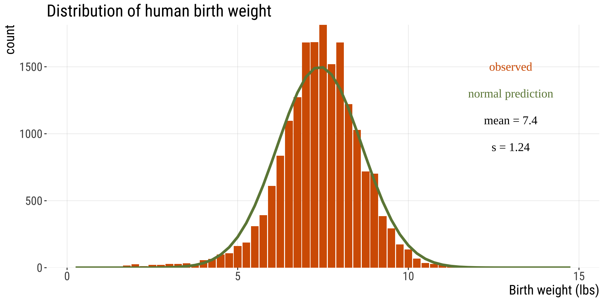
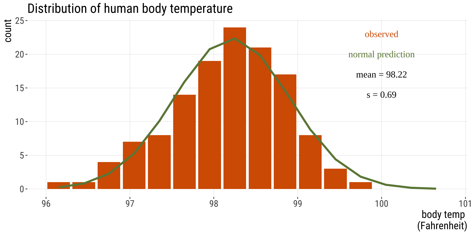
Human body temperature

• Body temp is (roughly) normally distributed

Data: Shoemaker (1996).“What’s Normal? – Temperature, Gender, and Heart Rate”

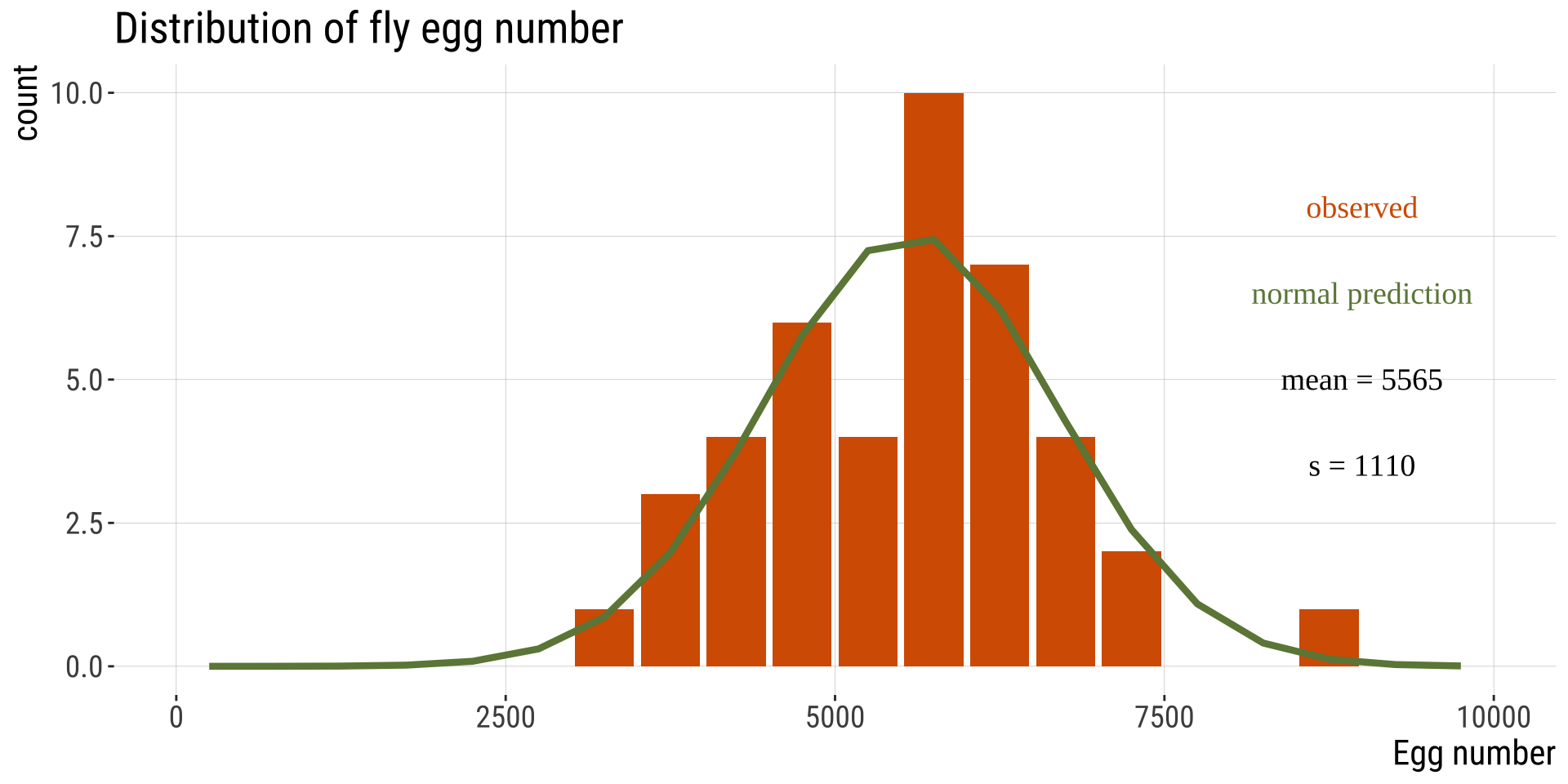
Drosophila egg number

• Drosophila egg number is (roughly) normally distributed

Paaby et al (2014). “A highly pleiotropic amino acid polymorphism in the Drosophila insulin receptor contributes to life-history adaptation”

The Normal Distribution: Definitions & Properties

Recap: Continuous probability distributions

• The probability of any one outcome from a continuous distribution, like the normal distribution, is infinitesimally small because there are infinite numbers in any range.
• We therefore describe continuous distributions with probability densities.
• Probability densities integrate to one: \[\int p_{x}=1\]

Warning: integrals! Don’t panic, you don’t need to integrate anything

The Normal Probability Density (1/)

• The probability density of each value \(x\) from a normal distribution with mean \(\mu\) and variance \(\sigma^2\) is:

\[f[x]=\frac{1}{\sqrt{2\pi\sigma^2}}e^{-\frac{(x-\mu)^2}{2\sigma^2}}\] * Thus, across sample space, probability densities integrate to 1, meaning

\[\int_{-\infty}^{+\infty}\frac{1}{\sqrt{2\pi\sigma^2}}e^{-\frac{(x-\mu)^2}{2\sigma^2}}=\int_{-\infty}^{+\infty}f(x)dx=1\] , meaning the integral of the PDF (probability density function) over its entire range integrates to 1.

Concept check in (1/2)

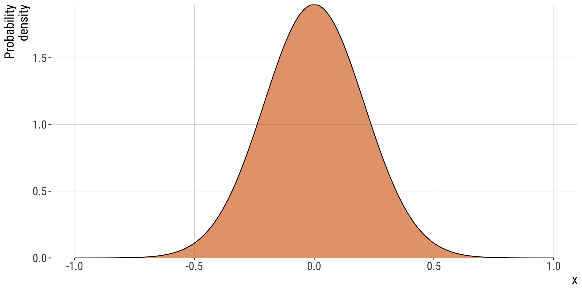
• This normal distribution has points with a probability density > 1.
• We know that probabilities cannot be greater than 1, so how can this be the case?

Concept check in (2/2)

• Answer: prob. densities integrate to one, aka the area under the curve, corresponding to probabilities. (i.e., \(\int p_{x}=1\)). Individual probability densities can exceed 1 though.
• Does this mean probability densities can be <1?
• Answer: No!The probability density function is non-negative for all possible values of the random variable. The total area under the probability density function is equal to 1.

Parameters of the Normal Distribution (1/2)

\(N(\mu, \sigma^2)\): These parameters - mean and variance (or standard deviation, \(\sigma\)) - fully specify a normal distribution

\(X\sim N(\mu, \sigma)\): \(X\) is normally distributed and the distribution is specified by a mean \(\mu\) and a standard deviation \(\sigma\)

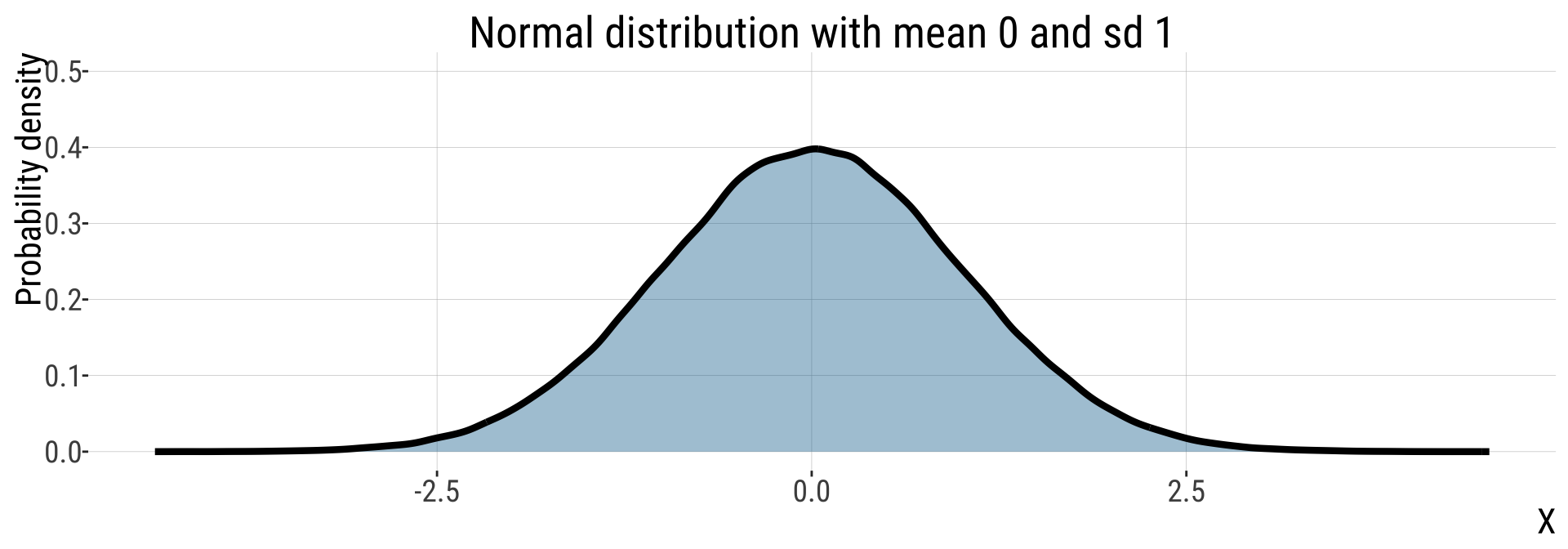
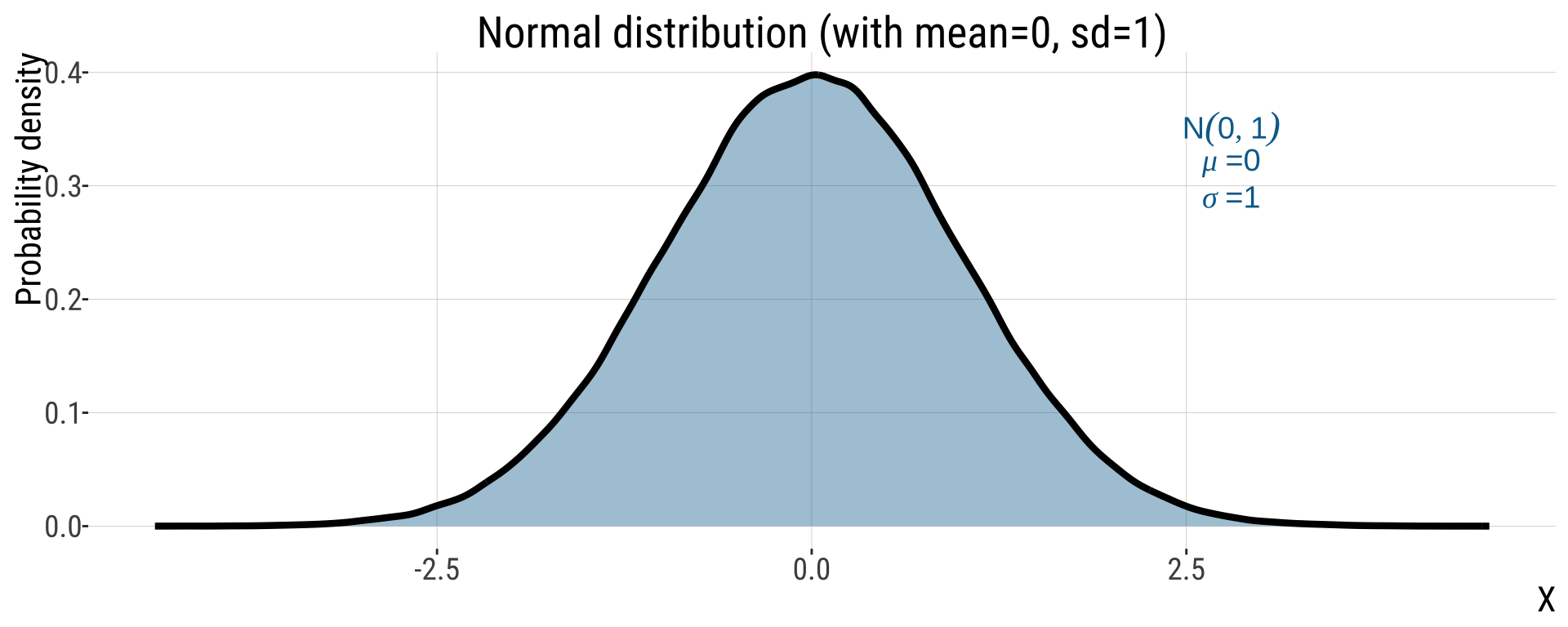
Parameters of the Normal Distribution (2/2)

• \(X\sim N(\mu, \sigma)\): \(X\) is normally distributed; normal is specified by \(\mu\) and \(\sigma\)

Visualizing Probability Densities

A Normal Distribution is symmetric around its mean

Properties of the normal

• The normal is symmetric around its mean
• The normal has a single mode
• The probability density is highest exactly at the mean.
• It follows that the mean, median, and mode are all equal to each other for the normal distribution!

Probability that \(X\) falls in a given range (1/2)

• Probability that \(X\) lies between two values, \(a\) and \(b\):

\[P[a<X<b]=\int_{a}^{b}\frac{1}{\sqrt{2\pi\sigma^2}}e^{-\frac{(x-\mu)^2}{2\sigma^2}}dx\]

Ouch…

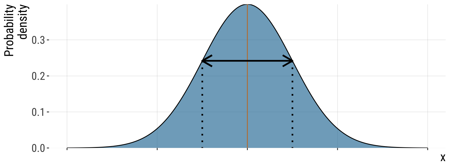
Probability that \(X\) falls in a given range (2/2)

• Some helpful (approximate) ranges:

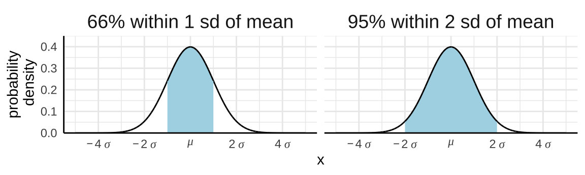
• These are approximations!

The standard normal distribution

A normal with \(\mu=0\) and \(\sigma=1\)

One Normal Distribution to Rule Them (1/2)

• Normal distributions can have distinct values of \(\mu\) and \(\sigma\) but must have the same shape.
• Of the infinite normal distributions, the standard normal distribution – a normal distribution with \(\mu=0\) and \(\sigma=1\) is particularly useful.

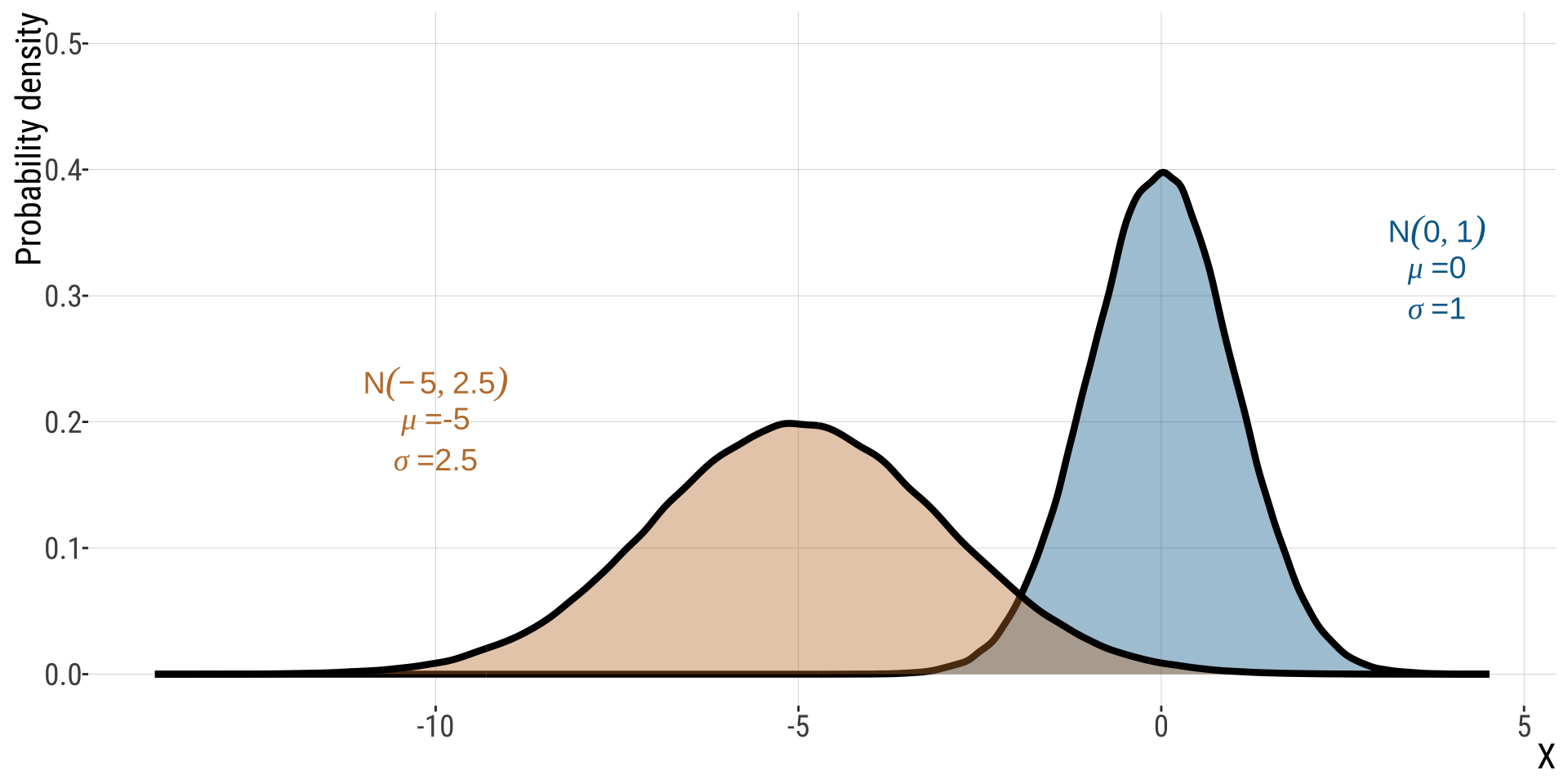
One Normal Distribution to Rule Them (2/2)

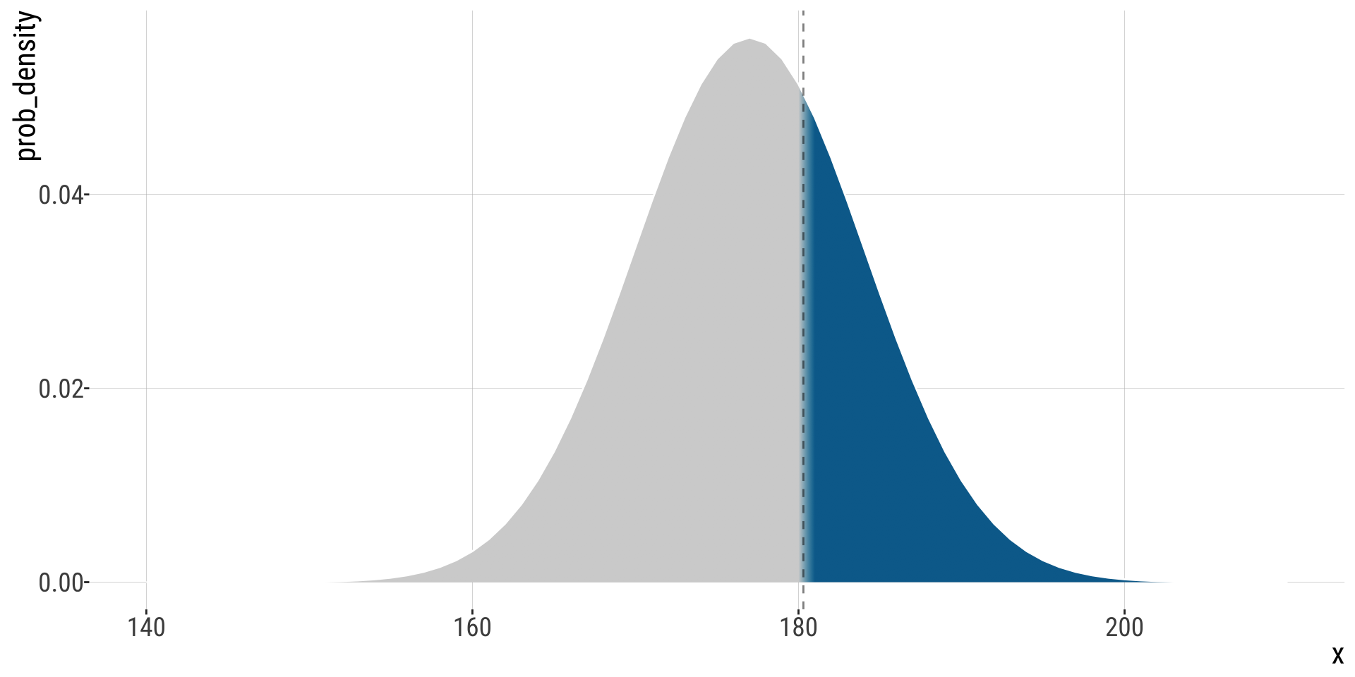
The \(Z\)-distribution

The \(Z\)-distribution describes the probability that a random draw from the standard normal is greater than a given value.

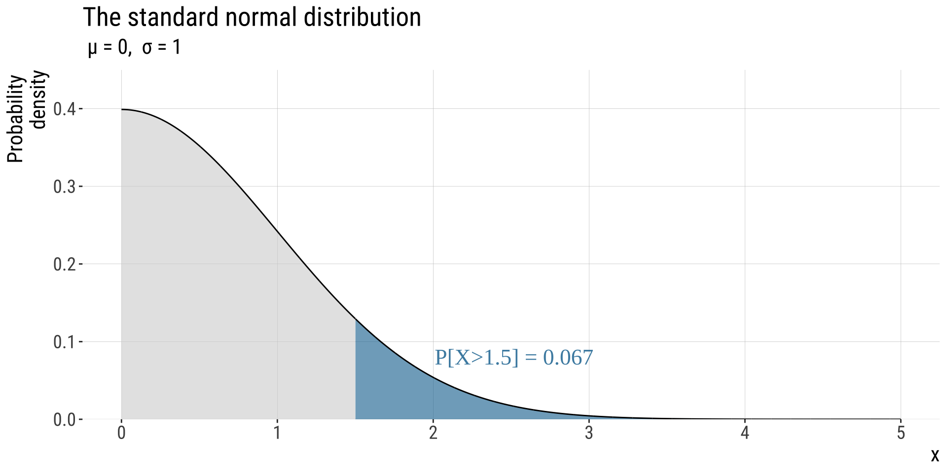
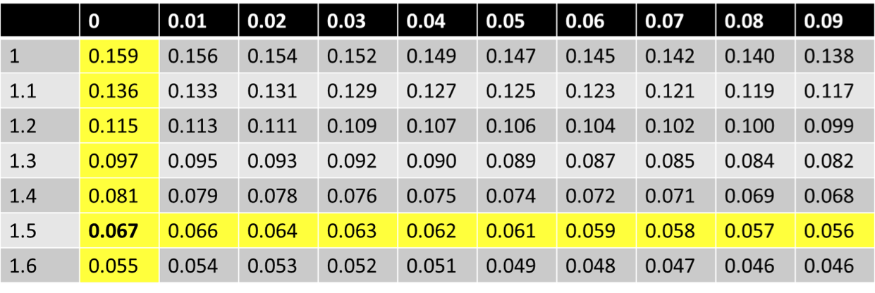
In R pnorm(x = 1.5, lower.tail = FALSE) = 0.067 In R: pnorm(q = 1.5, lower.tail = F): 0.0668

The Standard Normal Table (1/)

• We use the symbol \(Z\) to indicate a variable that has a standard normal distribution.
• The standard normal table: gives the probability of getting a random draw from a standard normal distribution greater than a given value

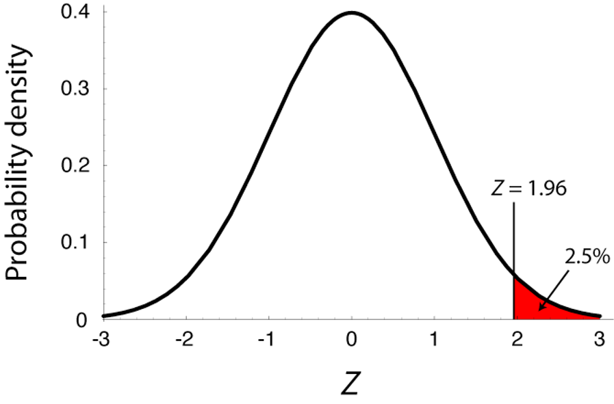
Figure 10.3-2 from textbook

The Standard Normal Table (2/)

• Rows contain the 1st two digits of Z
• Columns contain the 3rd digit
• The value is probability that a random draw from the standard normal is \(>Z\). E.g. \(P(Z>1.5)\)

Using the Z distribution

• The standard normal is symmetric about zero, so: \[𝑃[𝑋 < -Z]=P[Z > X]\], i.e. the probability that a random sample, \(X\), is less than \(-Z\) equals the probability that a random sample is greater than \(Z\).

• The normal integrates to one, so: \[P[X < Z]=1 − P[X > Z]\], i.e. the probability that a random sample is less than \(Z\) equals one minus the probability that a random sample is greater than \(Z\).

The Z transform

• Any normal distribution can be converted to the standard normal distribution by subtracting the population mean \(\mu\) from each value and dividing by the population standard deviation \(\sigma\):

\[Z=\frac{X-\mu}{\sigma}\] * E.g., by a \(Z\) transform, a value of \(X=0.4\) from a normal distribution with \(\mu=0.5\) and \(\sigma=0.1\) will be \(\frac{0.4-0.5}{0.1}=\frac{-0.1}{0.1}=-1\)

Z is called a “standard normal deviate”

Why use the Z transform?

• The \(Z\) transform is useful because we can then have a simple way to talk about results on a common scale.
• I think of a \(Z\) value as the number of standard deviations between an observation and the population mean.

\[Z=\frac{X-\mu}{\sigma}\]

• The benefits are similar to using the CV to compare standard deviations across different scales

• The other advantage: the standard Normal table

Example: British spies

British spies (1/)

• MI5 (the UK’s CIA) says a man has to be shorter than 180.3 cm tall to be a spy.
• Height of British men is normally distributed with mean 177.0 cm, and standard deviation 7.1cm.
• What proportion of British men are excluded from a career as a spy by this height criteria?

Let’s work on this!

British spies (2/)

• MI5 (the UK’s CIA) says a man has to be shorter than 180.3 cm tall to be a spy.
• Height of British men is normally distributed with mean 177.0 cm, and standard deviation 7.1cm.
• What proportion of British men are excluded from a career as a spy by this height criteria?

\(\mu=177\)

\(\sigma=7.1\)

What are we looking for? \(P[\text{height}>180.3|\mu=177,\sigma=7.1]=?\)

Make a rough sketch:

British spies (3/)

British spies (4/)

\[P[Z>180.3|\mu=177,\sigma=7.1]=?\]

1. \(Z\)-transform: \[(180.3-177)/7.1=0.46\]
2. Look this up in the standard normal table:

	0	0.01	0.02	0.03	0.04	0.05	0.06	0.07	0.08	0.09
0.3	0.382	0.378	0.374	0.371	0.367	0.363	0.359	0.356	0.352	0.348
0.4	0.345	0.341	0.337	0.334	0.330	0.326	0.323	0.319	0.316	0.312
0.5	0.309	0.305	0.302	0.298	0.295	0.291	0.288	0.284	0.281	0.278

Conclude that \(\sim 32.3\%\) of British men are too tall to be a spy.

British spies (4/)

# Probability of a random man in the UK being >= 180.3 cm tall.
pnorm(q = 180.3, mean = 177, sd = 7.1, lower.tail = FALSE)
## [1] 0.321

# probability of being <= 180.3 cm tall
pnorm(q = 180.3, mean = 177, sd = 7.1, lower.tail = TRUE)
## [1] 0.679

# or 1- P(>180.3)
1 - pnorm(q = 180.3, mean = 177, sd = 7.1, lower.tail = FALSE)
## [1] 0.679

The sampling distribution of means from samples taken from a normal distribution

Sample Means From a Normal

• Means of normally distributed variables are normally distributed.

\[\mu=\bar Y, \sigma_{\bar{Y}}=\frac{\sigma}{\sqrt{n}}\] - The mean of the sample means equals μ. The standard deviation of the sample means is the standard error, and equals \(\frac{\sigma}{\sqrt{n}}\)