3.2.Probability

Acknowledgments: many code snippets borrowed from Y. Brandvain

Bárbara D. Bitarello

2025-10-06

Outline

  • Definition(s) & Foundational Concepts
    • Probability vs. Odds
    • Probability as long-term frequency
    • Random trials
    • Types of events (exclusive and non-exclusive)
    • Probability distributions x probability densities x proportions
  • Probability rules
    • the addition principle
    • the general multiplication principle

Recap

Statistics and probability are not intuitive. Our brains do a bad job of interpreting data

  • we see patterns in random data
  • we tend to be overconfident
  • we tend to jump to conclusions
  • we don’t realize that coincidences are common
  • we have incorrect feelings about probability
  • we don’t expect variability to depend on sample size
  • we find it hard to combine probabilities (coming up soon)

To help us when generalizing from sample to population, we need Probability Theory: The foundation of statistical thinking

Definitions, Terminologies, and Notations

Why do we need probabilities?

We can use probability theory to connect sample estimates

  • Which we can obtain from data.
  • Which take their values by chance (variable).

To population parameters:

  • Which we can almost never obtain.
  • With values free from chance (population constant).

What is probability?

  • It depends.
  • Probability is super complex.
  • Entire books have been written on it and there are fiery debates about what even IS a probability.

Some definitions

  1. Probability “out there” - outside your head.

But also…

  1. Probability that is “inside your head” — as strength of subjective beliefs; may vary among people or even different assessments by the same person.

  2. “Probabilities” used to quantify ignorance – e.g. probability that a pregnant person is pregnant with a girl

  3. Quantitive predictions of one time events – e.g., presidential polls

Probability “out there” - outside your head

What we deal with in biology most of the time

  • This is probability as long-term frequency
  • The probability that a certain event will happen has a definite value (a parameter)
  • We rarely have enough data to know that value precisely (or good data to know it accurately), but we estimate it and give it different levels of confidence

Probability as long-term frequency

  • The probability of an event is its true relative frequency - “out there”

  • This is the proportion of times the event would occur if we repeated the same process over and over again

Example

Example: what’s the probability that a fair die will give me 2 if I roll it once?

  • This is probability as long-term frequency
  • It comes from the notion that if I could roll this die many, many times, I would get a 2 in about \(1/6\) of the times
  • So we say the answer here is \(1/6\)

Figure caption: figure 5.2-1 from the textbook.

Probability as long-term frequency

Two subtypes:

1) Probabilities as predictions from a model

  • e.g. odds of a baby being XY or XX is 50:50 based on meiosis alone

2) Probabilities based on data

  • in reality, long-term data cross many countries suggest odds of XY to XX baby are 51.7:50

Probability Theory & Statistics

Probabilities take values from 0-1 (or 0-100%)

They are used to quantify a prediction about a future event OR the certainty of a belief

A probability of zero (0%) indicates:

  • An event is impossible
    OR
  • Someone is absolutely (100%) sure that a statement is wrong

A probability of one (100%) indicates:

  • An event is certain to happen
    OR
  • Someone is absolutely (100%) sure that a statement is correct

A probability of 0.5 (50%) indicates:

  • An event is equally likely to happen or not happen
    OR
  • Someone believes that a statement is equally likely to be true or false

Lingo: Odds vs probability

  • They express the same thing
  • Probabilities can be expressed as odds
  • Odds can be expressed as probability
  • No consistency across fields and no advantage of one over the other
  • I learned and most often use “probability” - It sounds less ambiguous to me than odds, which people use more in normal parlance

Example: Sex ratio

Worldwide, the boy to girl sex ratio of babies born has been estimated to be 1.07. What is the probability of a random birth being a boy?

Odds: Probability that event will occur (male born) divided by probability it will not occur (female born). Can be any value 0 or positive (not negative).

  • Odds of having boy versus girl is:\(p[boy]/p[girl]=1.07\) – can also be phrased as \(1.07 \text{ to } 1\) or \(1.07:1\)

  • Equivalent to \(107 \text{ to } 100\) (\(107:100\)), \(1070 \text{ to } 1000\) (\(1070:1000\)), etc

Probability: if there are 107 boys born for every 100 girls, \(107/(100+107)=51.7\%\) or \(0.517\) is the probability of having a boy.

Foundational Concepts in Probability Theory

Random Trials

Example: Probability of getting a 4 in one roll (trial) of a six-sided die

  • A random trial is a process or experiment that has two or more possible outcomes whose occurrence cannot be predicted with certainty.

  • Only one outcome is observed from each repetition of a random trial.

Figure caption: figure 5.2-1 from the textbook.

Types of Events

Example: possible numbers in a die roll

Mutually Exclusive

If \(A\) and \(B\) are mutually exclusive:

  • Either \(A\) or \(B\) are individually plausible outcomes
  • \(A\&B\) is not plausible (i.e., \(P(A\&B)=0\))
Code
even_numbers <- c(2, 4, 6)
odd_numbers <- c(1, 3, 5)
l <- list(even = even_numbers, odd = odd_numbers, all = sort(c(even_numbers, odd_numbers)))
library(ggvenn)

p1 <- ggvenn(l[c(1:2)], fill_color = asteroidcity1(), show_elements = TRUE, text_size = 12) +
    ggtitle("Cannot be even AND odd") + theme(plot.title = element_text(family = "Roboto Condensed",
    size = 20))
p1

E.g., \(P(\text{even AND odd})=0\) in a die roll

Types of Events

Example: possible numbers in a die roll

Non-mutually exclusive

If \(A\) and \(B\) are not mutually exclusive:

  • There’s a chance of outcome \(A\) and \(B\)
  • I.e., it is plausible that \(P(A\&B)\neq0\)
Code
l2 <- list(even = even_numbers, prime = c(2, 3, 5))
p2 <- ggvenn(l2, fill_color = asteroidcity1(), show_elements = TRUE, text_size = 12) +
    ggtitle("Can be even AND prime") + theme(plot.title = element_text(family = "Roboto Condensed",
    size = 19))
p2

E.g., \(P(\text{even AND prime}) \neq 0\) in a die roll – in fact, what is it?

Probability distributions

A probability distribution is the true relative frequency of all possible values of a random variable.

Probability: Distributions vs. Densities

Probability distributions describe discrete variables.

Probability distributions sum to 1.

\(\sum{p[x]}=1\)

Code
ns <- rnorm(1e+06)
ggplot(tibble(x = ns), aes(x = x)) + geom_histogram(color = banff()[7], fill = "#00a1b7",
    bins = 30, alpha = 0.4) + ggtitle("Probability Distribution") + annotate("text",
    x = -4, y = 1e+05, parse = TRUE, label = "sum(P(x))==1", size = 4)

Code
# bb_theme()

Example: probability distribution for rolling a die

All possible values: \(x=\{1,2,3,4,5,6\}\)

Probabilities of particular outcomes: \(p[1]=1/6\)

\(p[2]=1/6,\text{etc}\)

Sum of probabilities of all possible outcomes:

\(\sum{p[x]}=1\)

Figure caption: figure 5.4-1 from the textbook.

Probability: Distributions vs. Densities

  • The probability of any value from a continuous distribution is infinitesimally small.

  • Probability densities integrate to 1.

\(\int{p[x]}=1\)

Code
ggplot(tibble(x = ns), aes(x = x)) + geom_density(fill = banff()[5], color = banff()[7],
    alpha = 0.8) + ggtitle("Probability Density") + annotate("text", x = -4, y = 0.3,
    parse = TRUE, label = "integral(f(x)*dx, a, b)", size = 4)

Example: the normal distribution!

Area under the curve gives you the probability of values in a range \(\left[a,b\right]\) Each value has an an infinitesimal probability value

Figure caption: figure 5.4-4 from the textbook.

Proportion

  • The proportion is the number of times an event occurs divided by the number of tries.

  • We can think of a proportion as a realized sample from our probability distribution.

Proportion: Outcome of a Die 🎲

Code
plot.one.dice.prob <- data.frame(outcome = c(1:6), probability = 1/6) |>
    ggplot(aes(x = outcome, y = probability, fill = factor(outcome))) + geom_bar(stat = "identity",
    show.legend = FALSE) + ggtitle("Probability Distribution", subtitle = "Outcome of a fair die") +
    scale_x_continuous(breaks = 1:6) + scale_y_continuous(expand = c(0, 0), limits = c(0,
    0.32)) + ylab("Expected probability") + bb_theme() + scale_fill_manual(values = banff()) +
theme(axis.ticks = element_blank())
df <- data.frame(Outcome = DieRoll(times = 6), NrRolls = 6)

one.roll <- ggplot(df, aes(x = Outcome, fill = factor(Outcome))) + geom_bar(aes(y = after_stat(count)/sum(count)),
    show.legend = FALSE) + ggtitle("Proportions Observed", subtitle = "Outcome of a fair die\n(n = 6 trials)") +
    scale_fill_manual(values = banff()) + scale_x_continuous(breaks = 1:12) + ylab(label = "Observed proportion") +
    theme(axis.ticks = element_blank())
library(patchwork)
plot.one.dice.prob + one.roll

The Sampling Distribution

The sampling distribution is the distribution of the parameter estimate of interest from these samples.

The sampling distribution is among the most important probability distributions for statistics.

Sampling Distribution 🎲

If we repeat die rolls a number of times, we can plot the proportions of {1,2,3,4,5,6} observed throughout many trials

Probability rules

  • The general multiplication principle

  • The general addition principle

The general addition principle (“this OR that”)

\(P[A \text{ OR } B]=P[A] + P[B] - P[A \text{ and } B]\)

Let’s practice

What is the probability of a die roll resulting in an even number OR a prime number?

\(P[A \text{ OR } B]\)

\(+P[A]\)

\(+P[B]\)

\(- P[A \text{ and }B]\)

Let’s practice

Even numbers: \(\{2,4,6\}\)

Prime numbers: \(\{2,3,5\}\)

Even and prime: \(\{2\}\)

\(P[\text{even}]=3/6=1/2\)

\(+P[\text{ prime}=3/6=1/2]\)

\(-P[\text{even AND prime} = 1-1/6=5/6\sim0.833\)

A special case of the addition principle

IF \(A\) and \(B\) are mutually exclusive, i.e., \(P[A \text{ AND } B]=0\), so:

Thus,

\(P[A \text{ OR } B]=P[A]+P[B]\)

Example 1: probability of a range

What is the probability the sum of two dice is between six and eight?

Code
plot.two.dice.prob <- data.frame(Outcome = factor(c(sapply(1:6, function(X) {
    X + 1:6
})))) |>
    ggplot(aes(x = Outcome)) + geom_bar(aes(y = after_stat(count)/sum(count)), group = 1,
    show.legend = FALSE) + ggtitle("Probability Distribution", subtitle = "Outcome of the sum of two fair dice") +
    scale_x_discrete(breaks = 1:12) + scale_y_continuous(expand = c(0, 0), limits = c(0,
    0.2)) + ylab("Expected probability") + bb_theme() + theme(axis.ticks = element_blank())
plot.two.dice.prob

Example 1 (cont.)

\(P[6]+P[7]+P[8] - P[6 \text{ AND } 7 \text{ AND } 8]\)

Code
data.frame(outcome = factor(c(2, 3, 4, 5, "6:8", 9, 10, 11, 12), levels = c(2, 3,
    4, 5, "6:8", 9, 10, 11, 12)), prob = c(1, 2, 3, 4, 5 + 6 + 5, 4, 3, 2, 1)/36) |>
    mutate(my.col = (outcome == "6:8")) |>
    ggplot(aes(x = outcome, y = prob, fill = my.col)) + geom_bar(stat = "identity",
    show.legend = FALSE) + ggtitle("Outcome of the sum of two fair dice") + scale_y_continuous(expand = c(0,
    0), limits = c(0, 0.5)) + bb_theme() + ylab("Expected probability") + scale_fill_manual(values = c("lightgray",
    "#006475")) + xlab(bquote(1^{
    st
} ~ +~2^{
    nd
} ~ roll)) + theme(axis.ticks = element_blank())

Example 2: probability of NOT

The probability the sum of two dice is not between six and eight.

We know that \(\sum{P[X]}=1\), so \(P[\text{ not }X]=1-P[X]\)

Code
dice7<-data.frame(outcome =  factor(c("Not between 6 & 8", "Between  6 & 8"), levels = c("Not between 6 & 8", "Between  6 & 8")),prob    =  c((1+2+3+4+4+3+2+1) , (5 +6+5) ) / 36)

dice7 |>
  mutate(my.col = (outcome == "6:8")) |>
  ggplot(aes(x = outcome, y = prob, fill = outcome)) +
  geom_bar(stat = "identity",show.legend = FALSE) +
  ggtitle("Outcome of the sum of two fair dice") +
  ylab("Expected probability") +
  scale_fill_manual(values = c("lightgray","#006475")) +
  scale_y_continuous(expand = c(0,0), limits  = c(0,.7))+ 
  bb_theme()+
  xlab(bquote(1^{st}~+~2^{nd}~roll))+
  theme(axis.ticks = element_blank())

Another example

Probability that the sum of two dice is odd or between 6 and 8.

Subtract P[A & B] to avoid double counting nonexclusive events

\(P[A \text{ or } B] = P[A] + P[B] - P[A \text{ and } B]\)

Code
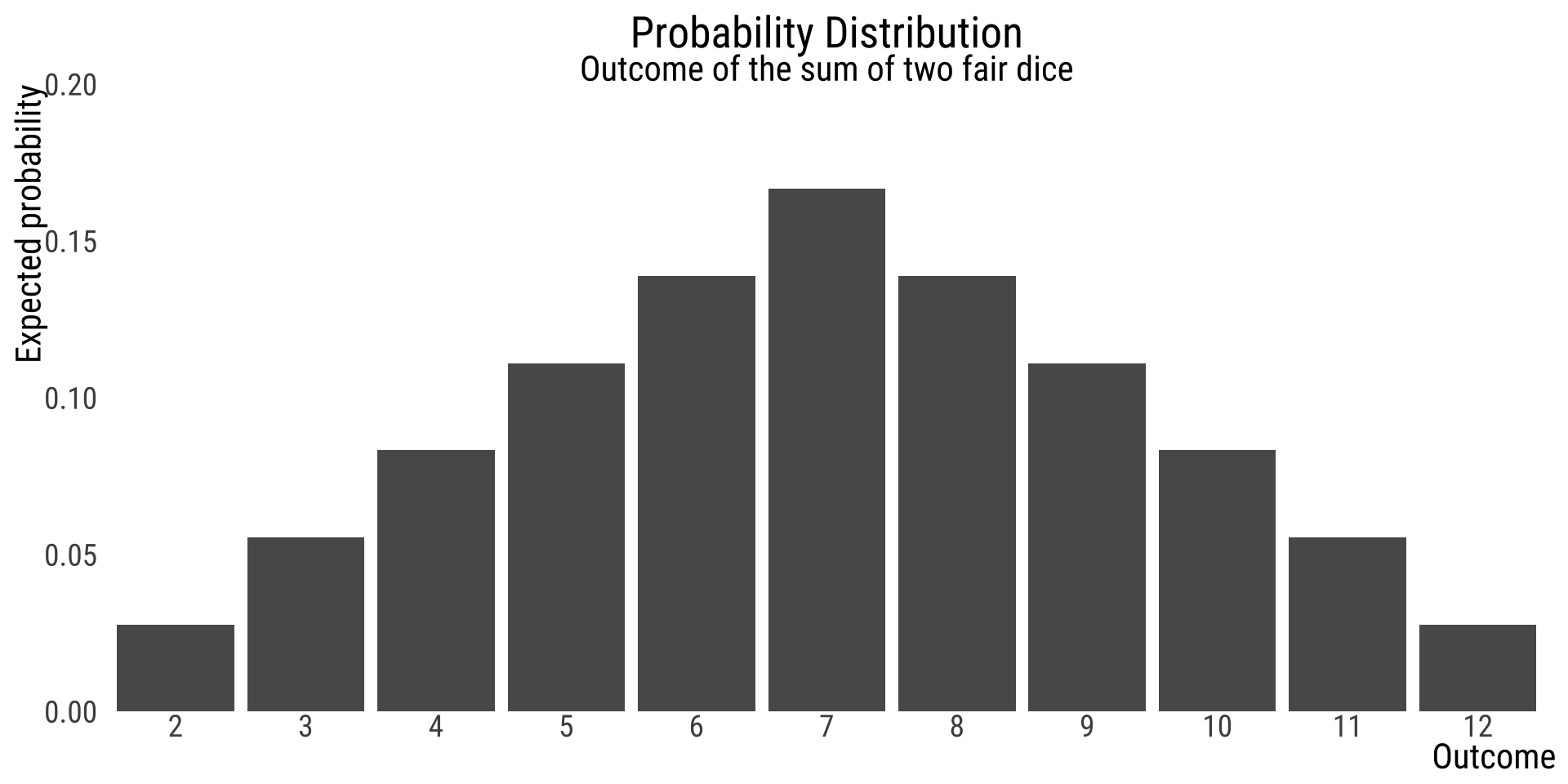
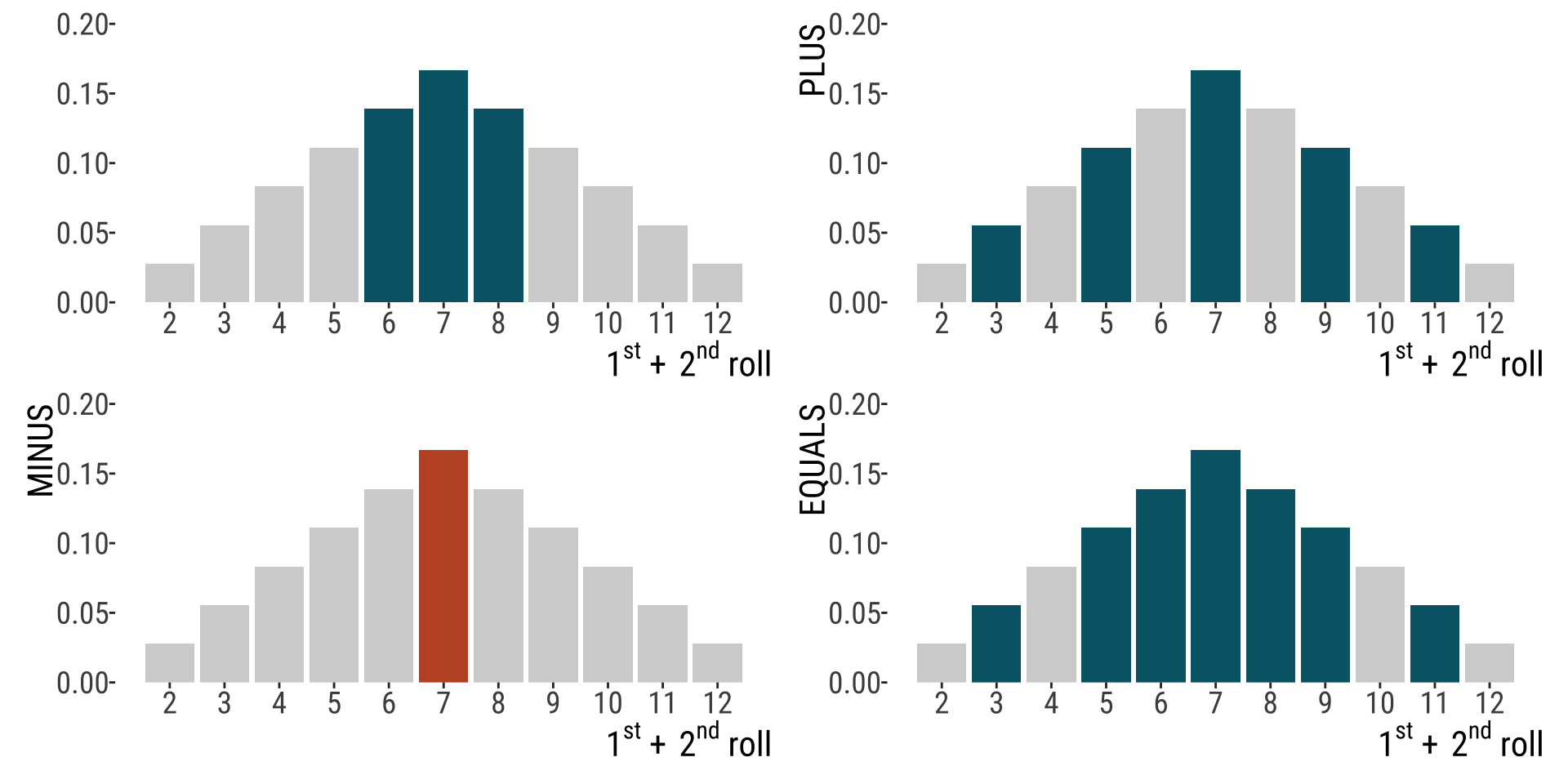
two.die.revisited <- data.frame(
  Outcome =  c(2, 3, 4, 5, 6, 7, 8, 9, 10, 11, 12),
  prob    =  c(1, 2, 3, 4, 5, 6, 5, 4, 3, 2, 1) / 36) |>
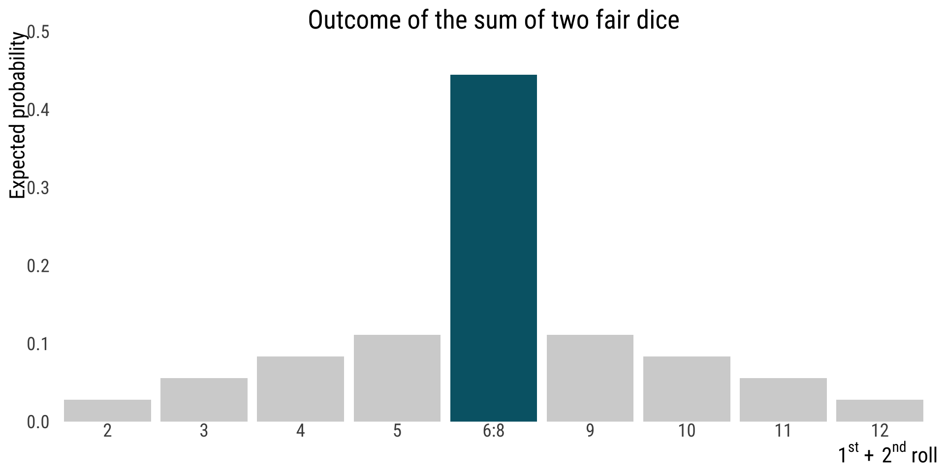
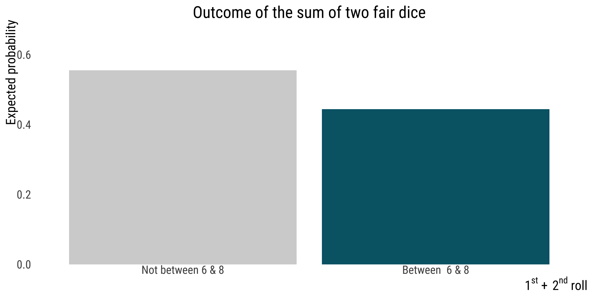
  mutate(sixeight = Outcome >5 & Outcome <9,
         odd      = Outcome %%2 ==1,
         oddandsixeight = sixeight &  odd, 
         oddorsixeight =  sixeight|odd)

dice.theme <- ggplot(two.die.revisited, aes(x = Outcome, y = prob)) +
  ylab("")+
  scale_y_continuous(expand = c(0,0), limits  = c(0,.2))+ 
  scale_x_continuous(breaks = 1:12) +
  bb_theme() +
 xlab(bquote(1^{st}~+~2^{nd}~roll))


sixthrougheight <- dice.theme +  
  geom_bar(aes(fill = sixeight),stat = "identity",show.legend = FALSE) + 
  scale_fill_manual(values = c("lightgray","#006475")) 

odd <- dice.theme +  
  geom_bar(aes(fill = odd),stat = "identity",show.legend = FALSE) +
  scale_fill_manual(values = c("lightgray","#006475"))+ 
  ylab("PLUS")

seven <- dice.theme +  
  geom_bar(aes(fill = oddandsixeight),stat = "identity",show.legend = FALSE) +
  scale_fill_manual(values = c("lightgray","#C0532B"))+ 
  ylab("MINUS")
tots <- dice.theme +  
  geom_bar(aes(fill = oddorsixeight),
           stat = "identity",show.legend = FALSE) + scale_fill_manual(values = c("lightgray","#006475"))+ 
  ylab("EQUALS")  

library(patchwork)
sixthrougheight+ odd+ seven+ tots

That’s all for today

"Forrest says "And that's all I wanted to say about that"

From: makeameme.org